Custom and special datasets
Continual Learning Datasets
Toy (Regression) Problems
2D Donut Dataset
This data handler creates a synthetic toy problem comprising 2D annuli.
- class hypnettorch.data.special.donuts.Donuts(centers=((0, 0), (0, 0)), radii=((3, 4), (9, 10)), num_train=100, num_test=100, use_one_hot=True, rseed=42)[source]
Bases:
DatasetDonut dataset handler.
Note, each donut prescribes a different class.
- Parameters:
centers (tuple or list) – List of tuples, each determining the center of a donut.
radii (tuple or list) – List of tuples, each tuple defines the inner and outer radius of a donut.
num_train (int) – Number of training samples per donut.
num_test (int) – Number of test samples per donut.
use_one_hot (bool) – Whether the class labels should be represented as a one-hot encoding.
rseed (int) – If
None, the current random state of numpy is used to generate the data. Otherwise, a new random state with the given seed is generated.
- plot_dataset(title, show=True, filename=None, interactive=False, figsize=(10, 6))[source]
Plot samples belonging to this dataset.
- Parameters:
(....) – See docstring of method
data.dataset.Dataset.plot_samples().
 satisfiying:
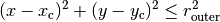

Gaussian Mixture via a set of Gaussian Datasets
The module data.special.gaussian_mixture_data contains a toy dataset
consisting of input data drawn from a 2D Gaussian distribution. Combining
several such datasets creates a Gaussian mixture (e.g., each mixture component
would be one dataset from class GaussianData).
- The dataset is inspired by the toy example provided in section 4.5 of
However, the mixture of Gaussians only determines the input domain x (which is enough for a GAN dataset). Though, we also need to specify the output y.
For instance, each Gaussian bump could be the input domain of one task. Given this input domain, the task would be to predict p(x), thus y = p(x).
In the case of small variances, the task can be detected from seeing the input x alone. This allows us to predict task embeddings based on inputs, such that there is no need to define the task embedding manually.
- class hypnettorch.data.special.gaussian_mixture_data.GaussianData(mean=array([0, 0]), cov=array([[0.0025, 0.0], [0.0, 0.0025]]), num_train=100, num_test=100, map_function=None, rseed=None)[source]
Bases:
DatasetAn instance of this class shall represent a regression task where the input samples
 are drawn from a Gaussian with given mean and
variance.
are drawn from a Gaussian with given mean and
variance.Due to plotting functionalities, this class only supports 2D inputs and 1D outputs.
Generate a new dataset.
The input data x for train and test samples will be drawn iid from the given Gaussian. Per default, the map function is the probability density of the given Gaussian: y = f(x) = p(x).
- Parameters:
mean – The mean of the Gaussian.
cov – The covariance of the Gaussian.
num_train – Number of training samples.
num_test – Number of test samples.
map_function (optional) – A function handle that receives input samples and maps them to output samples. If not specified, the density function will be used as map function.
rseed (int) – If
None, the current random state of numpy is used to generate the data. Otherwise, a new random state with the given seed is generated.
- property cov
Covariance matrix.
- property mean
Mean vector.
- plot_dataset(show=True)[source]
Plot the whole dataset.
- Parameters:
show (bool) – Whether the plot should be shown.
- Returns:
The figure handle.
- static plot_datasets(data_handlers, inputs=None, predictions=None, labels=None, show=True, filename=None, figsize=(10, 6))[source]
Plot several datasets of this class in one plot.
- Parameters:
data_handlers – A list of GaussianData objects.
inputs (optional) – A list of numpy arrays representing inputs for each dataset.
predictions (optional) – A list of numpy arrays containing the predicted output values for the given input values.
labels (optional) – A label for each dataset.
show – Whether the plot should be shown.
filename (optional) – If provided, the figure will be stored under this filename.
figsize – A tuple, determining the size of the figure in inches.
- plot_predictions(predictions, label='Pred', show_train=True, show_test=True)[source]
Plot the dataset as well as predictions.
- Parameters:
predictions – A tuple of x and y values, where the y values are computed by a trained regression network. Note, that x is supposed to be 2D numpy array, whereas y is a 1D numpy array.
label – Label of the predicted values as shown in the legend.
show_train – Show train samples.
show_test – Show test samples.
- plot_samples(title, inputs, outputs=None, predictions=None, num_samples_per_row=4, show=True, filename=None, interactive=False, figsize=(10, 6))[source]
Plot samples belonging to this dataset.
Note
Either
outputsorpredictionsmust be notNone!- Parameters:
title – The title of the whole figure.
inputs – A 2D numpy array, where each row is an input sample.
outputs (optional) – A 2D numpy array of actual dataset targets.
predictions (optional) – A 2D numpy array of predicted output samples (i.e., output predicted by a neural network).
num_samples_per_row – Maximum number of samples plotted per row in the generated figure.
show – Whether the plot should be shown.
filename (optional) – If provided, the figure will be stored under this filename.
interactive – Turn on interactive mode. We mainly use this option to ensure that the program will run in background while figure is displayed. The figure will be displayed until another one is displayed, the user closes it or the program has terminated. If this option is deactivated, the program will freeze until the user closes the figure. Note, if using the iPython inline backend, this option has no effect.
figsize – A tuple, determining the size of the figure in inches.
- hypnettorch.data.special.gaussian_mixture_data.get_gmm_tasks(means=[array([-4, -4]), array([-4, -2]), array([-4, 0]), array([-4, 2]), array([-4, 4]), array([-2, -4]), array([-2, -2]), array([-2, 0]), array([-2, 2]), array([-2, 4]), array([0, -4]), array([0, -2]), array([0, 0]), array([0, 2]), array([0, 4]), array([2, -4]), array([2, -2]), array([2, 0]), array([2, 2]), array([2, 4]), array([4, -4]), array([4, -2]), array([4, 0]), array([4, 2]), array([4, 4])], covs=[array([[0.0025, 0.0], [0.0, 0.0025]]), array([[0.0025, 0.0], [0.0, 0.0025]]), array([[0.0025, 0.0], [0.0, 0.0025]]), array([[0.0025, 0.0], [0.0, 0.0025]]), array([[0.0025, 0.0], [0.0, 0.0025]]), array([[0.0025, 0.0], [0.0, 0.0025]]), array([[0.0025, 0.0], [0.0, 0.0025]]), array([[0.0025, 0.0], [0.0, 0.0025]]), array([[0.0025, 0.0], [0.0, 0.0025]]), array([[0.0025, 0.0], [0.0, 0.0025]]), array([[0.0025, 0.0], [0.0, 0.0025]]), array([[0.0025, 0.0], [0.0, 0.0025]]), array([[0.0025, 0.0], [0.0, 0.0025]]), array([[0.0025, 0.0], [0.0, 0.0025]]), array([[0.0025, 0.0], [0.0, 0.0025]]), array([[0.0025, 0.0], [0.0, 0.0025]]), array([[0.0025, 0.0], [0.0, 0.0025]]), array([[0.0025, 0.0], [0.0, 0.0025]]), array([[0.0025, 0.0], [0.0, 0.0025]]), array([[0.0025, 0.0], [0.0, 0.0025]]), array([[0.0025, 0.0], [0.0, 0.0025]]), array([[0.0025, 0.0], [0.0, 0.0025]]), array([[0.0025, 0.0], [0.0, 0.0025]]), array([[0.0025, 0.0], [0.0, 0.0025]]), array([[0.0025, 0.0], [0.0, 0.0025]])], num_train=100, num_test=100, map_functions=None, rseed=None)[source]
Generate a set of data handlers (one for each task) of class
GaussianData.- Parameters:
means – The mean of each Gaussian.
covs – The covariance matrix of each Gaussian.
num_train – Number of training samples per task.
num_test – Number of test samples per task.
map_functions (optional) – A list of “map_functions”, one for each task.
rseed (int) – See argument
rseedof classGaussianData. Thei-th dataset generated by this function will be passed the the random staterseed+iis specified.
- Returns:
A list of objects of class
GaussianData.- Return type:
(list)
Gaussian Mixture Model Dataset
The module data.special.gaussian_mixture_data is stemming from a
conditional view, where every mode in the Gaussian mixture is a separate task
(single dataset). Therefore, it provides N distinct data handlers when
having N distinct modes.
Unfortunately, this configuration is not ideal for unsupervised GAN training (as we want to be able to provide batches that contain data from a mix of modes without having to manually assemble these batches) or for training a classifier for a GMM toy problem.
Therefore, this module provides a wrapper that converts a sequence of data
handlers of class data.special.gaussian_mixture_data.GaussianData
(i.e., a set of single modes) to a combined data handler.
Model description:
Let denote the input data. The class GMMData assumes that
it’s input training data is drawn from the following Gaussian Mixture Model:
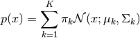
with mixing coefficients  , such that
  .
.
Note, it is up to the user of this class to provide appropriate training data
(only important to keep in mind if unequal train set sizes are provided via
constructor argument gaussian_datasets or if mixing_coefficients are
non-uniform).
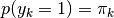
Let  denote a
  -dimensional 1-hot encoding, i.e.,
 and
and  . Thus, is the
latent variable that we want to infer (e.g., the optimal classification label)
with marginal probabilities:
. Thus, is the
latent variable that we want to infer (e.g., the optimal classification label)
with marginal probabilities:
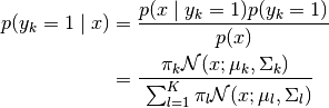
The conditional likelihood of a component is:

Using Bayes Theorem we obtain the posterior:
- class hypnettorch.data.special.gmm_data.GMMData(gaussian_datasets, classification=False, use_one_hot=False, mixing_coefficients=None)[source]
Bases:
DatasetDataset with inputs drawn from a Gaussian mixture model.
An instance of this class combines several instances of class
data.special.gaussian_mixture_data.GaussianDatainto one data handler. I.e., multiple gaussian bumps are combined to a Gaussian mixture dataset.Most importantly, the dataset can be turned into a classification task, where the label corresponds to the ID of the Gaussian bump from which the sample was drawn. Otherwise, the original outputs will remain.
Note
You can use function
data.special.gaussian_mixture_data.get_gmm_tasks()to create a set of tasks to be passed as constructor argumentgaussian_datasets.- Parameters:
gaussian_datasets (list) – A list of instances of class
data.special.gaussian_mixture_data.GaussianData.classification (bool) – If
True, the original outputs of the datasets will be omitted and replaced by the dataset index. Therefore, the original regression datasets are combined to a single classification dataset.use_one_hot (bool) – Whether the class labels should be represented as a one-hot encoding. This option only applies if
classificationisTrue.mixing_coefficients (list, optional) –
The mixing coefficients
of the individual mixture components. If not
specified, will be assumed to be
1. / self.num_modes.Note
Mixing coefficients have to sum to
1.Note
If mixing coefficients are not uniform, then one has to externally ensure that the training data is distributed accordingly. For instance, if
mixing_coefficients=[.1, .9], then the second dataset passed viagaussian_datasetsshould have 9 times more training samples then the first dataset.
- estimate_distance(fake, component_densities=None, density_estimation='hist', eps=1e-05)[source]
This method estimates the distance/divergence of the empirical fake distribution with the underlying true data disctribution.
Therefore, we utilize the fact that we know the data distribution.
The following distance/divergence measures are implemented:
Symmetric KL divergence: The fake samples are used to estimate the model density. The fake samples are used to estimate
 . An additional
set of real samples is drawn from the training data to compute a
Monte Carlo estimate of
. An additional
set of real samples is drawn from the training data to compute a
Monte Carlo estimate of
 .
.Comment from Simone Surace about this approach: “Doing density estimation first and then computing the integral is known to be the wrong way to go (there is an entire literature about this problem).” This should be kept in mind when using this estimate.
- Parameters:
fake (numpy.ndarray) – A 2D numpy array, where each row is an input sample (usually drawn from a generator network).
component_densities (numpy.ndarray, optional) – A 2D numpy array with each row corresponding to a sample in
fakeand each column corresponding to a mode in this dataset. Each entry represents the density of the corresponding sample under the corresponding mixture component. See return valueresponsibilitiesof methodestimate_mode_coverage().density_estimation –
Which kind of method should be used to estimate the model distribution (i.e., density of given samples under the distribution estimated from those samples). Available methods are:
'hist': We estimate the fake density based on a normalized 2D histogram of the samples. We use the Square-root choice to compute the number of bins per dimension.'gaussian': Uses the kernel density method'gaussian'fromsklearn.neighbors.kde.KernelDensity. Note, we don’t change the default`bandwidth`value!
eps (float) – We don’t allow densities to be smaller than this value for numerical stability reasons (when computing the log).
- Returns:
The estimated symmetric KL divergence.
- estimate_mode_coverage(fake, responsibilities=None)[source]
Compute the mode coverage of fake samples as suggested in
This method will compute the responsibilities for each fake sample towards each mixture component and assign each sample to the mixture component with the highest responsibility. Mixture components that get no fake sample assigned are considered dropped modes.
The paper referenced above used 10,000 fake samples (on their synthetic dataset) to measure the mode coverage.
- Parameters:
fake – A 2D numpy array, where each row is an input sample (usually drawn from a generator network).
responsibilities (optional) – The responsibilities of each fake data point (may be unnormalized). A 2D numpy array with each row corresponding to a sample in fake and each column corresponding to a mode in this dataset.
- Returns:
A tuple containing:
num_covered: The number of modes that have at least one fake sample with maximum responsibility being assigned to that mode.
responsibilities: The given or computed responsibilities. If computed by this method, the responsibilities will be unnormalized, i.e., correspond to the densities per component of this mixture model.
- Return type:
(tuple)
- get_input_mesh(x1_range=None, x2_range=None, grid_size=1000)[source]
Create a 2D grid of input values.
The default grid returned by this method will also be the default grid used by the method
plot_uncertainty_map().Note
This method is only implemented for 2D datasets.
- Parameters:
x1_range (tuple, optional) –
The min and max value for the first input dimension. If not specified, the range will be automatically inferred.
Automatical inference is based on the underlying data (train and test). The range will be set, such that all data can be drawn inside.
x2_range (tuple, optional) – Same as
x1_rangefor the second input dimension.grid_size (int or tuple) – How many input samples per dimension. If an integer is passed, then the same number grid size will be used for both dimension. The grid is build by equally spacing
grid_sizeinside the rangesx1_rangeandx2_range.
- Returns:
Tuple containing:
x1_grid (numpy.ndarray): A 2D array, containing the grid values of the first dimension.
x2_grid (numpy.ndarray): A 2D array, containing the grid values of the second dimension.
flattended_grid (numpy.ndarray): A 2D array, containing all samples from the first dimension in the first column and all values corresponding to the second dimension in the second column. This format correspond to the input format as, for instance, returned by methods such as
data.dataset.Dataset.get_train_inputs().
- Return type:
(tuple)
- property means
2D array, containing the mean of each component in its rows.
- Type:
np.ndarray
- plot_optimal_classification(title='Classification Map', input_mesh=None, mesh_modes=None, sample_inputs=None, sample_modes=None, sample_label=None, sketch_components=False, show=True, filename=None, figsize=(10, 6))[source]
Plot a color-coded grid on how to optimally classify for each input value.
Note
Since the training data is drawn randomly, it might be that some training samples have a label that doesn’t correpond to the optimal label.
- Parameters:
(....) – See arguments of method
plot_uncertainty_map().mesh_modes (numpy.ndarray, optional) – If not provided, then the color of each grid position
is determined based on
 .
Otherwise, the labeling provided here will determine the
coloring.
.
Otherwise, the labeling provided here will determine the
coloring.
- plot_real_fake(title, real, fake, show=True, filename=None, interactive=False, figsize=(10, 6))[source]
Useful method when using this dataset in conjunction with GAN training. Plots the given real and fake input samples in a 2D plane.
- Parameters:
(....) – See docstring of method
data.dataset.Dataset.plot_samples().real (numpy.ndarray) – A 2D numpy array, where each row is an input sample. These samples correspond to actual input samples drawn from the dataset.
fake (numpy.ndarray) – A 2D numpy array, where each row is an input sample. These samples correspond to generated samples.
- plot_samples(title, inputs, outputs=None, predictions=None, show=True, filename=None, interactive=False, figsize=(10, 6))[source]
Plot samples belonging to this dataset.
- Parameters:
(....) – See docstring of method
data.dataset.Dataset.plot_samples().
- plot_uncertainty_map(title='Uncertainty Map', input_mesh=None, uncertainties=None, use_generative_uncertainty=False, use_ent_joint_uncertainty=False, sample_inputs=None, sample_modes=None, sample_label=None, sketch_components=False, norm_eps=None, show=True, filename=None, figsize=(10, 6))[source]
Draw an uncertainty heatmap.
- Parameters:
title (str) – Title of plots.
input_mesh (tuple, optional) – The input mesh of the heatmap (see return value of method
get_input_mesh()). If not specified, the default return value of methodget_input_mesh()is used.uncertainties (numpy.ndarray, optional) –
The uncertainties corresponding to
input_mesh. If not specified, then the uncertainties will be computed based the entropy across for
for
Note
The entropies will be normalized by the maximum uncertainty
-np.log(1.0 / self.num_modes).use_generative_uncertainty (bool) – If
True, the uncertainties plotted by default (ifuncertaintiesis left unspecified) are not based on the entropy of the responsibilities , but are the densities of the
underlying GMM
, but are the densities of the
underlying GMM  .
.use_ent_joint_uncertainty (bool) –
If
True, the uncertainties plotted by default (ifuncertaintiesis left unspecified) are based on the entropy of at location
:
at location
: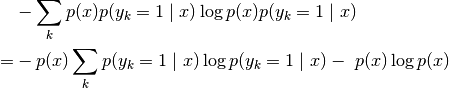
Note, we normalize
by its maximum inside the chosen
grid. Hence, the plot depends on the chosen input_mesh. In this way,![p(x) \in [0, 1]](_images/math/ec5f231fae06c5b657e3fc5f507b31bf9dd67643.png) and the second term
and the second term
![-p(x) \log p(x) \in [0, \exp(-1)]](_images/math/ddad680f5f052acccdb6028aa1598723fa6b7d1a.png) (note,
(note,
 would be negative for
  ).
).The first term is simply the entropy of
 scaled by . Hence, it shows where in the input space
are the regions where Gaussian bumps are overlapping (regions
in which data exists but multiple labels are
possible).
scaled by . Hence, it shows where in the input space
are the regions where Gaussian bumps are overlapping (regions
in which data exists but multiple labels are
possible).The second term shows the boundaries of the data manifold. Note,
 and
and
 .
.Note
This option is mutually exclusive with option
use_generative_uncertainty.Note
Entropies of
won’t be normalized in this
case.sample_inputs (numpy.ndarray, optional) – Sample inputs. Can be specified if a scatter plot of samples (e.g., train samples) should be laid above the heatmap.
sample_modes (numpy.ndarray, optional) – To which mode do the samples in
sample_inputsbelong to? If provided, then for each sample insample_inputsa number smaller thannum_modesis expected. All samples with the same mode identifier are colored with the same color.sample_label (str, optional) – If a label should be shown in the legend for inputs
sample_inputs.sketch_components (bool) – Sketch the mean and variance of each component.
norm_eps (float, optional) – If uncertainties are computed by this method, then (normalized) densities for each x-value in the input mesh have to be computed. To avoid division by zero, a positive number
norm_epscan be specified.(....) – See docstring of method
data.dataset.Dataset.plot_samples().
1D Regression Dataset
The module data.special.regression1d_data contains a data handler for a
CL toy regression problem. The user can construct individual datasets with this
data handler and use each of these datasets to train a model in a continual
leraning setting.
- class hypnettorch.data.special.regression1d_data.ToyRegression(train_inter=[-10, 10], num_train=20, test_inter=[-10, 10], num_test=80, val_inter=None, num_val=None, map_function=<function ToyRegression.<lambda>>, std=0.0, perturb_test_val=False, rseed=None)[source]
Bases:
DatasetAn instance of this class shall represent a simple regression task.
Generate a new dataset.
The input data x will be uniformly drawn for train samples and equidistant for test samples. The user has to specify a function that will map this random input data onto output samples y.
- Parameters:
A tuple, representing the interval from which x samples are drawn in the training set.
train_intermay also be provided as a list of tuples, in which case training samples will be distributed according to the range covered by each tuple.num_train (int) – Number of training samples.
test_inter (tuple) – A tuple, representing the interval from which x samples are drawn in the test set.
num_test (int) – Number of test samples.
val_inter (tuple, optional) – See parameter test_inter. If set, this argument leads to the construction of a validation set. Note, option
num_valneed to be specified as well.num_val (int, optional) – Number of validation samples.
map_function (func) – A function handle that receives input samples and maps them to output samples.
std (float or func) –
If not zero, Gaussian white noise with this std will be added to the training outputs.
Heteroscedasticity can be realized by passing a function
 that describes the standard deviations at a
given location . Note, this function may only outputs
numbers
that describes the standard deviations at a
given location . Note, this function may only outputs
numbers  .
.perturb_test_val (bool) – By default, the option
stdonly adds noise to the training data, not the validation or test data. If this option isTrue, then also the validation and test targets will be perturbed. This might be helpful for measuring calibration.rseed (int) – If
None, the current random state of numpy is used to generate the data. Otherwise, a new random state with the given seed is generated.
- plot_dataset(show=True)[source]
Plot the whole dataset.
- Parameters:
show – Whether the plot should be shown.
- static plot_datasets(data_handlers, inputs=None, predictions=None, labels=None, fun_xranges=None, show=True, filename=None, figsize=(10, 6), publication_style=False)[source]
Plot several datasets of this class in one plot.
- Parameters:
data_handlers – A list of ToyRegression objects.
inputs (optional) – A list of numpy arrays representing inputs for each dataset.
predictions (optional) – A list of numpy arrays containing the predicted output values for the given input values.
labels (optional) – A label for each dataset.
fun_xranges (optional) – List of x ranges in which the true underlying function per dataset should be sketched.
show – Whether the plot should be shown.
filename (optional) – If provided, the figure will be stored under this filename.
figsize – A tuple, determining the size of the figure in inches.
publication_style – Whether the plots should be in publication style.
- plot_predictions(predictions, label='Pred', show_train=True, show_test=True)[source]
Plot the dataset as well as predictions.
- Parameters:
predictions – A tuple of x and y values, where the y values are computed by a trained regression network. Note, that we assume the x values to be sorted.
label – Label of the predicted values as shown in the legend.
show_train – Show train samples.
show_test – Show test samples.
- plot_samples(title, inputs, outputs=None, predictions=None, num_samples_per_row=4, show=True, filename=None, interactive=False, figsize=(10, 6))[source]
Plot samples belonging to this dataset.
Note
Either
outputsorpredictionsmust be notNone!- Parameters:
title – The title of the whole figure.
inputs – A 2D numpy array, where each row is an input sample.
outputs (optional) – A 2D numpy array of actual dataset targets.
predictions (optional) – A 2D numpy array of predicted output samples (i.e., output predicted by a neural network).
num_samples_per_row – Maximum number of samples plotted per row in the generated figure.
show – Whether the plot should be shown.
filename (optional) – If provided, the figure will be stored under this filename.
interactive – Turn on interactive mode. We mainly use this option to ensure that the program will run in background while figure is displayed. The figure will be displayed until another one is displayed, the user closes it or the program has terminated. If this option is deactivated, the program will freeze until the user closes the figure. Note, if using the iPython inline backend, this option has no effect.
figsize – A tuple, determining the size of the figure in inches.
- property test_x_range
The input range for test samples.
- property train_x_range
The input range for training samples.
- property val_x_range
The input range for validation samples.
1D Regression Dataset with bimodal error
The module data.special.regression1d_bimodal_data contains a data handler
for a CL toy regression problem. The user can construct individual datasets with
this data handler and use each of these datasets to train a model in a continual
learning setting.
- class hypnettorch.data.special.regression1d_bimodal_data.BimodalToyRegression(train_inter=[-10, 10], num_train=20, test_inter=[-10, 10], num_test=80, val_inter=None, num_val=None, map_function=<function BimodalToyRegression.<lambda>>, alpha1=0.5, dist1=5, dist2=None, std1=1, std2=None, rseed=None, perturb_test_val=False)[source]
Bases:
ToyRegressionAn instance of this class shall represent a simple regression task, but with a bimodal Gaussian mixture error distribution.
Generate a new dataset.
The input data x will be uniformly drawn for train samples and equidistant for test samples. The user has to specify a function that will map this random input data onto output samples y.
- Parameters:
(....) – See docstring of class
data.special.regression_1d_data.ToyRegression.alpha1 – Mixture coefficient of the first Gaussian mode of the error.
dist1 – The distance from zero of mean of the first Gaussian component of the error.
dist2 (optional) – The distance from zero of mean of the first Gaussian component of the error. If
None, the value of dist1 will be taken.std1 – The standard deviation of the first Gaussian component of the error.
std2 (optional) – The standard deviation of the first Gaussian component of the error. If
None, the value of std1 will be taken.
Classification Tasks
Permuted MNIST Dataset
The module data.special.permuted_mnist contains a data handler for the
permuted MNIST dataset.
- class hypnettorch.data.special.permuted_mnist.PermutedMNIST(data_path, use_one_hot=True, validation_size=0, permutation=None, padding=0, trgt_padding=None)[source]
Bases:
MNISTDataAn instance of this class shall represent the permuted MNIST dataset, which is the same as the MNIST dataset, just that input pixels are shuffled by a random matrix.
Note
Image transformations are computed on the fly when transforming batches to torch tensors. Hence, this class is only applicable to PyTorch applications. Internally, the class stores the unpermuted images.
- Parameters:
data_path – Where should the dataset be read from? If not existing, the dataset will be downloaded into this folder.
use_one_hot – Whether the class labels should be represented in a one-hot encoding.
validation_size – The number of validation samples. Validation samples will be taking from the training set (the first
 samples).
permutation – The permutation that should be applied to the dataset. If
None, no permutation will be applied. We expect a numpy permutation of the formnp.random.permutation((28+2*padding)**2)padding –
The amount of padding that should be applied to images.
Note
The padding is currently not reflected in the :attr:`data.dataset.Dataset.in_shape attribute, as the padding is only applied to torch tensors. See attribute
torch_in_shape.trgt_padding (int, optional) – If provided,
trgt_paddingfake classes will be added, such that in total the returned dataset haslen(labels) + trgt_paddingclasses. However, all padded classes have no input instances. Note, that 1-hot encodings are padded to fit the new number of classes.
- input_to_torch_tensor(x, device, mode='inference', force_no_preprocessing=False, sample_ids=None)[source]
This method can be used to map the internal numpy arrays to PyTorch tensors.
Note, this method has been overwritten from the base class.
It applies zero padding and pixel permutations.
- Parameters:
(....) – See docstring of method
data.dataset.Dataset.input_to_torch_tensor().- Returns:
The given input
xas PyTorch tensor.- Return type:
- property permutation
The permuation matrix that is applied to input images before they are transformed to Torch tensors.
- tf_input_map(mode='inference')[source]
Not implemented! The class currently does not support Tensorflow.
- property torch_in_shape
The input shape of images, similar to attribute in_shape. In contrast to in_shape, this attribute reflects the padding that is applied when calling
classifier.permuted_mnist.PermutedMNIST.input_to_torch_tensor().
- class hypnettorch.data.special.permuted_mnist.PermutedMNISTList(permutations, data_path, use_one_hot=True, validation_size=0, padding=0, trgt_padding=None, show_perm_change_msg=True)[source]
Bases:
objectA list of permuted MNIST tasks that only uses a single instance of class
PermutedMNIST.An instance of this class emulates a Python list that holds objects of class
PermutedMNIST. However, it doesn’t actually hold several objects, but only one with just the permutation matrix being exchanged everytime a different element of this list is retrieved. Therefore, use this class with care!As all list entries are the same PermutedMNIST object, one should never work with several list entries at the same time! -> Retrieving a new list entry will modify every previously retrieved list entry!
When retrieving a slice, a shallow copy of this object is created (i.e., the underlying
PermutedMNISTdoes not change) with only the desired subgroup of permutations avaliable.
Why would one use this object? When working with many permuted MNIST tasks, then the memory consumption becomes significant if one desires to hold all task instances at once in working memory. An object of this class only needs to hold the MNIST dataset once in memory. Just the number of permutation matrices grows linearly with the number of tasks.
Caution
You may never use more than one entry of this class at the same time, as all entries share the same underlying data object and therewith the same permutation.
Note
The mini-batch generation process is maintained separately for every permutation. Thus, the retrieval of mini-batches for different permutations does not influence one another.
Example
You should never use this list as follows
dhandlers = PermutedMNISTList(permutations, '/tmp')
d0 = dhandlers[0]
# Zero-th permutation is active ...
# ...
d1 = dhandlers[1]
# First permutation is active for `d0` and `d1`!
# Important, you may not use `d0` anymore, as this might lead to
# undesired behavior.
Example
Instead, always work with only one list entry at a time. The following usage would be correct
dhandlers = PermutedMNISTList(permutations, '/tmp')
d = dhandlers[0]
# Zero-th permutation is active ...
# ...
d = dhandlers[1]
# First permutation is active for `d` as expected.
- Parameters:
(....) – See docstring of constructor of class
PermutedMNIST.permutations – A list of permutations (see parameter
permutationof classPermutedMNISTto have a description of valid list entries). The length of this list denotes the number of tasks.show_perm_change_msg – Whether to print a notification everytime the data permutation has been exchanged. This should be enabled during developement such that a proper use of this list is ensured. Note You may never work with two elements of this list at a time.
Split MNIST Dataset
The module data.special.split_mnist contains a wrapper for data
handlers for the SplitMNIST task.
- class hypnettorch.data.special.split_mnist.SplitMNIST(data_path, use_one_hot=False, validation_size=1000, use_torch_augmentation=False, labels=[0, 1], full_out_dim=False, trgt_padding=None)[source]
Bases:
MNISTDataAn instance of the class shall represent a SplitMNIST task.
- Parameters:
data_path (str) – Where should the dataset be read from? If not existing, the dataset will be downloaded into this folder.
use_one_hot (bool) – Whether the class labels should be represented in a one-hot encoding.
validation_size (int) – The number of validation samples. Validation samples will be taking from the training set (the first
samples).use_torch_augmentation (bool) – See docstring of class
data.mnist_data.MNISTData.labels (list) – The labels that should be part of this task.
full_out_dim (bool) – Choose the original MNIST instead of the new task output dimension. This option will affect the attributes
data.dataset.Dataset.num_classesanddata.dataset.Dataset.out_shape.trgt_padding (int, optional) – If provided,
trgt_paddingfake classes will be added, such that in total the returned dataset haslen(labels) + trgt_paddingclasses. However, all padded classes have no input instances. Note, that 1-hot encodings are padded to fit the new number of classes.
- transform_outputs(outputs)[source]
Transform the outputs from the 10D MNIST dataset into proper labels based on the constructor argument
labels.I.e., the output will have
len(labels)classes.Example
Split with labels [2,3]
1-hot encodings: [0,0,0,1,0,0,0,0,0,0] -> [0,1]
labels: 3 -> 1
- Parameters:
outputs – 2D numpy array of outputs.
- Returns:
2D numpy array of transformed outputs.
- hypnettorch.data.special.split_mnist.get_split_mnist_handlers(data_path, use_one_hot=True, validation_size=0, use_torch_augmentation=False, num_classes_per_task=2, num_tasks=None, trgt_padding=None)[source]
This function instantiates 5 objects of the class
SplitMNISTwhich will contain a disjoint set of labels.The SplitMNIST task consists of 5 tasks corresponding to the images with labels [0,1], [2,3], [4,5], [6,7], [8,9].
- Parameters:
data_path – Where should the MNIST dataset be read from? If not existing, the dataset will be downloaded into this folder.
use_one_hot – Whether the class labels should be represented in a one-hot encoding.
validation_size – The size of the validation set of each individual data handler.
use_torch_augmentation (bool) – See docstring of class
data.mnist_data.MNISTData.num_classes_per_task (int) – Number of classes to put into one data handler. If
2, then every data handler will include 2 digits.num_tasks (int, optional) – The number of data handlers that should be returned by this function.
trgt_padding (int, optional) – See docstring of class
SplitMNIST.
- Returns:
A list of data handlers, each corresponding to a
SplitMNISTobject.- Return type:
(list)
Split CIFAR-10/100 Dataset
The module data.special.split_cifar contains a wrapper for data handlers
for the Split-CIFAR10/CIFAR100 task.
- class hypnettorch.data.special.split_cifar.SplitCIFAR100Data(data_path, use_one_hot=False, validation_size=1000, use_data_augmentation=False, use_cutout=False, labels=range(0, 10), full_out_dim=False)[source]
Bases:
CIFAR100DataAn instance of the class shall represent a single SplitCIFAR-100 task.
- Parameters:
data_path – Where should the dataset be read from? If not existing, the dataset will be downloaded into this folder.
use_one_hot (bool) – Whether the class labels should be represented in a one-hot encoding.
validation_size – The number of validation samples. Validation samples will be taking from the training set (the first
samples).use_data_augmentation (optional) – Note, this option currently only applies to input batches that are transformed using the class member
data.dataset.Dataset.input_to_torch_tensor()(hence, only available for PyTorch). Note, we are using the same data augmentation pipeline as for CIFAR-10.use_cutout (bool) – See docstring of class
data.cifar10_data.CIFAR10Data.labels – The labels that should be part of this task.
full_out_dim – Choose the original CIFAR instead of the the new task output dimension. This option will affect the attributes
data.dataset.Dataset.num_classesanddata.dataset.Dataset.out_shape.
- transform_outputs(outputs)[source]
Transform the outputs from the 100D CIFAR100 dataset into proper labels based on the constructor argument
labels.See
data.special.split_mnist.SplitMNIST.transform_outputs()for more information.- Parameters:
outputs – 2D numpy array of outputs.
- Returns:
2D numpy array of transformed outputs.
- class hypnettorch.data.special.split_cifar.SplitCIFAR10Data(data_path, use_one_hot=False, validation_size=1000, use_data_augmentation=False, use_cutout=False, labels=range(0, 2), full_out_dim=False)[source]
Bases:
CIFAR10DataAn instance of the class shall represent a single SplitCIFAR-10 task.
Each instance will contain only samples of CIFAR-10 belonging to a subset of the labels.
- Parameters:
(....) – See docstring of class
SplitCIFAR100Data.
- transform_outputs(outputs)[source]
Transform the outputs from the 10D CIFAR10 dataset into proper labels based on the constructor argument
labels.See
data.special.split_mnist.SplitMNIST.transform_outputs()for more information.- Parameters:
outputs (numpy.ndarray) – 2D numpy array of outputs.
- Returns:
2D numpy array of transformed outputs.
- Return type:
- hypnettorch.data.special.split_cifar.get_split_cifar_handlers(data_path, use_one_hot=True, validation_size=0, use_data_augmentation=False, use_cutout=False, num_classes_per_task=10, num_tasks=6)[source]
This method will combine 1 object of the class
data.cifar10_data.CIFAR10Dataand 5 objects of the classSplitCIFAR100Data.The SplitCIFAR benchmark consists of 6 tasks, corresponding to the images in CIFAR-10 and 5 tasks from CIFAR-100 corresponding to the images with labels [0-10], [10-20], [20-30], [30-40], [40-50].
- Parameters:
data_path – Where should the CIFAR-10 and CIFAR-100 datasets be read from? If not existing, the datasets will be downloaded into this folder.
use_one_hot (bool) – Whether the class labels should be represented in a one-hot encoding.
validation_size – The size of the validation set of each individual data handler.
use_data_augmentation (optional) – Note, this option currently only applies to input batches that are transformed using the class member
data.dataset.Dataset.input_to_torch_tensor()(hence, only available for PyTorch).use_cutout (bool) – See docstring of class
data.cifar10_data.CIFAR10Data.num_classes_per_task (int) –
Number of classes to put into one data handler. For example, if
2, then every data handler will include 2 digits.If
10, then the first dataset will simply be CIFAR-10.num_tasks (int) – A number between 1 and 11 (assuming
num_classes_per_task == 10), specifying the number of data handlers to be returned. Ifnum_tasks=6, then there will be the CIFAR-10 data handler and the first 5 splits of the CIFAR-100 dataset (as in the usual CIFAR benchmark for CL).
- Returns:
(list) A list of data handlers. The first being an instance of class
data.cifar10_data.CIFAR10Dataand the remaining ones being an instance of classSplitCIFAR100Data.