Utilities and helper functions 

This subpackage contains common helper functions to a variety of problems (e.g., PyTorch checkpointing, special layers, computing diagonal Fisher matrices, …).

Batch Normalization 

Implementation of a hypernet compatible batchnorm layer.

The joint use of batch-normalization and hypernetworks is not straight forward, mainly due to the statistics accumulated by the batch-norm operation which expect the weights of the main network to only change slowly. If a hypernetwork replaces the whole set of weights, the statistics previously estimated by the batch-norm layer might be completely off.

To circumvent this problem, we provide multiple solutions:

In a continual learning setting with one set of weights per task, we can simply estimate and store statistics per task (hence, the batch-norm operation has to be conditioned on the task).

The statistics are distilled into the hypernetwork. This would require the addition of an extra loss term.

The statistics can be treated as parameters that are outputted by the hypernetwork. In this case, nothing enforces that these “statistics” behave similar to statistics that would result from a running estimate (hence, the resulting operation might have nothing in common with batch- norm).

Always use the statistics estimated on the current batch.

Note, we also provide the option of turning off the statistics, in which case the statistics will be set to zero mean and unit variance. This is helpful when interpreting batch-normalization as a general form of gain modulation (i.e., just applying a shift and scale to neural activities).

class hypnettorch.utils.batchnorm_layer.BatchNormLayer(num_features, momentum=0.1, affine=True, track_running_stats=True, frozen_stats=False, learnable_stats=False)[source]

Bases: Module

Hypernetwork-compatible batch-normalization layer.

Note, batch normalization performs the following operation

$y = \frac{x - \mathrm{E}[x]}{\sqrt{\mathrm{Var}[x] + \epsilon}} * \ \gamma + \beta$

This class allows to deviate from this standard implementation in order to provide the flexibility required when using hypernetworks. Therefore, we slightly change the notation to

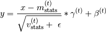
$y = \frac{x - m_{\text{stats}}^{(t)}}{\sqrt{v_{\text{stats}}^{(t)} + \ \epsilon}} * \gamma^{(t)} + \beta^{(t)}$

We use this notation to highlight that the running statistics $m_{\text{stats}}^{(t)}$ and $v_{\text{stats}}^{(t)}$ are not necessarily estimates resulting from mean and variance computation but might be learned parameters (e.g., the outputs of a hypernetwork).

We additionally use the superscript $(t)$ to denote that the gain $\gamma$ , offset $\beta$ and statistics may be dynamically selected based on some external context information.

This class provides the possibility to checkpoint statistics $m_{\text{stats}}^{(t)}$ and $v_{\text{stats}}^{(t)}$ , but not gains and offsets.

Note

If context-dependent gains $\gamma^{(t)}$ and offsets $\beta^{(t)}$ are required, then they have to be maintained externally, e.g., via a task-conditioned hypernetwork (see this paper for an example) and passed to the forward() method.

Parameters:

num_features – See argument num_features, for instance, of class torch.nn.BatchNorm1d.
momentum – See argument momentum of class torch.nn.BatchNorm1d.
affine –
See argument affine of class torch.nn.BatchNorm1d. If set to False, the input activity will simply be “whitened” according to the applied layer statistics (except if gain $\gamma$ and offset $\beta$ are passed to the forward() method).

Note, if learnable_stats is False, then setting affine to False results in no learnable weights for this layer (running stats might still be updated, but not via gradient descent).

Note, even if this option is False, one may still pass a gain $\gamma$ and offset $\beta$ to the forward() method.
track_running_stats – See argument track_running_stats of class torch.nn.BatchNorm1d.
frozen_stats –
If True, the layer statistics are frozen at their initial values of $\gamma = 1$ and $\beta = 0$ , i.e., layer activity will not be whitened.

Note, this option requires track_running_stats to be set to False.
learnable_stats –
If True, the layer statistics are initialized as learnable parameters (requires_grad=True).

Note, these extra parameters will be maintained internally and not added to the weights. Statistics can always be maintained externally and passed to the forward() method.

Note, this option requires track_running_stats to be set to False.

checkpoint_stats(device=None)[source]

Buffers for a new set of running stats will be registered.

Calling this function will also increment the attribute num_stats.

Parameters:: device (optional) – If not provided, the newly created statistics will either be moved to the device of the most recent statistics or to CPU if no prior statistics exist.

forward(inputs, running_mean=None, running_var=None, weight=None, bias=None, stats_id=None)[source]

Apply batch normalization to given layer activations.

Based on the state if this module (attribute training), the configuration of this layer and the parameters currently passed, the behavior of this function will be different.

The core of this method still relies on the function torch.nn.functional.batch_norm(). In the following we list the different behaviors of this method based on the context.

In training mode:

We first consider the case that this module is in training mode, i.e., torch.nn.Module.train() has been called.

Usually, during training, the running statistics are not used when computing the output, instead the statistics computed on the current batch are used (denoted by use batch stats in the table below). However, the batch statistics are typically updated during training (denoted by update running stats in the table below).

The above described scenario would correspond to passing batch statistics to the function torch.nn.functional.batch_norm() and setting the parameter training to True.

training mode	use batch stats	update running stats
given stats	Yes	Yes
track running stats	Yes	Yes
frozen stats	No	No
learnable stats	Yes	Yes [1]
no track running stats	Yes	No

The meaning of each row in this table is as follows:

given stats: External stats are provided via the parameters running_mean and running_var.

track running stats: If track_running_stats was set to True in the constructor and no stats were given.

frozen stats: If frozen_stats was set to True in the constructor and no stats were given.

learnable stats: If learnable_stats was set to True in the constructor and no stats were given.

no track running stats: If none of the above options apply, then the statistics will always be computed from the current batch (also in eval mode).

Note

If provided, running stats specified via running_mean and running_var always have priority.

In evaluation mode:

We now consider the case that this module is in evaluation mode, i.e., torch.nn.Module.eval() has been called.

Here is the same table as above just for the evaluation mode.

evaluation mode	use batch stats	update running stats
track running stats	No	No
frozen stats	No	No
learnable stats	No	No
given stats	No	No
no track running stats	Yes	No

Parameters:

inputs – The inputs to the batchnorm layer.
running_mean (optional) –
Running mean stats $m_{\text{stats}}$ . This option has priority, i.e., any internally maintained statistics are ignored if given.

Note

If specified, then running_var also has to be specified.
running_var (optional) –
Similar to option running_mean, but for the running variance stats $v_{\text{stats}}$

Note

If specified, then running_mean also has to be specified.
weight (optional) – The gain factors $\gamma$ . If given, any internal gains are ignored. If option affine was set to False in the constructor and this option remains None, then no gains are multiplied to the “whitened” inputs.
bias (optional) – The behavior of this option is similar to option weight, except that this option represents the offsets $\beta$ .
stats_id –
This argument is optional except if multiple running stats checkpoints exist (i.e., attribute num_stats is greater than 1) and no running stats have been provided to this method.

Note

This argument is ignored if running stats have been passed.

Returns:

The layer activation inputs after batch-norm has been applied.

get_stats(stats_id=None)[source]

Get a set of running statistics (means and variances).

Parameters:

stats_id (optional) – ID of stats. If not provided, the most recent stats are returned.

Returns:

Tuple containing:

running_mean
running_var

Return type:

(tuple)

property hyper_shapes

A list of list of integers. Each list represents the shape of a weight tensor that can be passed to the forward() method. If all weights are maintained internally, then this attribute will be None.

Specifically, this attribute is controlled by the argument affine. If affine is True, this attribute will be None. Otherwise this attribute contains the shape of $\gamma$ and $\beta$ .

Type:: list or None

property num_stats

The number $T$ of internally managed statistics $\{(m_{\text{stats}}^{(1)}, v_{\text{stats}}^{(1)}), \dots, \ (m_{\text{stats}}^{(T)}, v_{\text{stats}}^{(T)}) \}$ . This number is incremented everytime the method checkpoint_stats() is called.

Type:: int

property param_shapes

A list of list of integers. Each list represents the shape of a parameter tensor.

Note, this attribute is independent of the attribute weights, it always comprises the shapes of all weight tensors as if the network would be stand-alone (i.e., no weights being passed to the forward() method). Note, unless learnable_stats is enabled, the layer statistics are not considered here.

Type:: list

training: bool

property weights

A list of all internal weights of this layer. If all weights are assumed to be generated externally, then this attribute will be None.

Type:: list or None

Common command-line arguments 

This file has a collection of helper functions that can be used to specify command-line arguments. In particular, arguments that are necessary for multiple experiments (even though with different default values) should be specified here, such that we do not define arguments (and their help texts) multiple times.

All functions specified here are helper functions for a simulation specific argument parser such as cifar.train_args.parse_cmd_arguments().

Important note for contributors 

DO NEVER CHANGE DEFAULT VALUES. Instead, add a keyword argument to the corresponding method, that allows you to change the default value, when you call the method.

hypnettorch.utils.cli_args.check_invalid_argument_usage(args)[source]

This method checks for common conflicts when using the arguments defined by methods in this module.

The following things will be checked:

Based on the optimizer choices specified in train_args(), we assert here that only one optimizer is selected at a time.

Assert that clip_grad_value and clip_grad_norm are not set at the same time.

Assert that split_head_cl3 is only set for cl_scenario=3

Assert that the arguments specified in function main_net_args() are correctly used.

Note

The checks can’t handle prefixes yet.

Parameters:: args – The parsed command-line arguments, i.e., the output of method argparse.ArgumentParser.parse_args().
Raises:: ValueError – If invalid argument combinations are used.

hypnettorch.utils.cli_args.cl_args(parser, show_beta=True, dbeta=0.01, show_from_scratch=False, show_multi_head=False, show_cl_scenario=False, show_split_head_cl3=True, dcl_scenario=1, show_num_tasks=False, dnum_tasks=1, show_num_classes_per_task=False, dnum_classes_per_task=2, show_calc_hnet_reg_targets_online=False, show_hnet_reg_batch_size=False, dhnet_reg_batch_size=-1)[source]

This is a helper method of the method parse_cmd_arguments to add an argument group for typical continual learning arguments.

Arguments specified in this function:

beta
train_from_scratch
multi_head
cl_scenario
split_head_cl3
num_tasks
num_classes_per_task
calc_hnet_reg_targets_online
hnet_reg_batch_size

Parameters:

parser – Object of class argparse.ArgumentParser.
show_beta – Whether option beta should be shown.
dbeta – Default value of option beta.
show_from_scratch – Whether option train_from_scratch should be shown.
show_multi_head – Whether option multi_head should be shown.
show_cl_scenario – Whether option cl_scenario should be shown.
show_split_head_cl3 – Whether option split_head_cl3 should be shown. Only has an effect if show_cl_scenario is True.
dcl_scenario – Default value of option cl_scenario.
show_num_tasks – Whether option num_tasks should be shown.
dnum_tasks – Default value of option num_tasks.
show_num_classes_per_task – Whether option show_num_classes_per_task should be shown.
dnum_classes_per_task – Default value of option dnum_classes_per_task.
show_calc_hnet_reg_targets_online (bool) – Whether the option calc_hnet_reg_targets_online should be provided.
show_hnet_reg_batch_size (bool) – Whether the option hnet_reg_batch_size should be provided.
dhnet_reg_batch_size (int) – Default value of option hnet_reg_batch_size.

Returns:

The created argument group, in case more options should be added.

hypnettorch.utils.cli_args.data_args(parser, show_disable_data_augmentation=False, show_data_dir=False, ddata_dir='.')[source]

This is a helper method of the function parse_cmd_arguments to add an argument group for typical dataset related options.

Arguments specified in this function:

disable_data_augment

Parameters:

parser – Object of class argparse.ArgumentParser.
show_disable_data_augmentation (bool) – Whether option disable_data_augmentation should be shown.
show_data_dir (bool) – Whether option data_dir should be shown.
ddata_dir (str) – Default value of option data_dir.

Returns:

The created argument group, in case more options should be added.

hypnettorch.utils.cli_args.eval_args(parser, dval_iter=500, show_val_batch_size=False, dval_batch_size=256, show_val_set_size=False, dval_set_size=0, show_test_with_val_set=False)[source]

This is a helper method of the method parse_cmd_arguments to add an argument group for validation and testing options.

Arguments specified in this function:

val_iter
val_batch_size
val_set_size
test_with_val_set

Parameters:

parser – Object of class argparse.ArgumentParser.
dval_iter (int) – Default value of argument val_iter.
show_val_batch_size (bool) – Whether the val_batch_size argument should be shown.
dval_batch_size (int) – Default value of argument val_batch_size.
show_val_set_size (bool) – Whether the val_set_size argument should be shown.
dval_set_size (int) – Default value of argument val_set_size.
show_test_with_val_set (bool) – Whether the test_with_val_set argument should be shown.

Returns:

The created argument group, in case more options should be added.

hypnettorch.utils.cli_args.gan_args(parser)[source]

This is a helper method of the method parse_cmd_arguments to add an argument group for options to configure the generator and discriminator network.

Deprecated since version 1.0: Please use method main_net_args() and generator_args() instead.

Parameters:: parser – Object of class argparse.ArgumentParser.
Returns:: The created argument group, in case more options should be added.

hypnettorch.utils.cli_args.generator_args(agroup, dlatent_dim=3)[source]

This is a helper method of the method parse_cmd_arguments (or more specifically an auxillary method to train_args()) to add arguments to an argument group for options specific to a main network that should act as a generator.

Arguments specified in this function:

latent_dim
latent_std

Parameters:

agroup – The argument group returned by, for instance, function main_net_args().
dlatent_dim – Default value of option latent_dim.

hypnettorch.utils.cli_args.hnet_args(parser, allowed_nets=['hmlp'], dhmlp_arch='100,100', show_cond_emb_size=True, dcond_emb_size='8', dchmlp_chunk_size=1000, dchunk_emb_size=8, show_use_cond_chunk_embs=True, dhdeconv_shape='512,512,3', prefix=None, pf_name=None, **kwargs)[source]

This is a helper function to add an argument group for hypernetwork- specific arguments to a given argument parser.

Arguments specified in this function:

hnet_type
hmlp_arch
cond_emb_size
chmlp_chunk_size
chunk_emb_size
use_cond_chunk_embs
hdeconv_shape
hdeconv_num_layers
hdeconv_filters
hdeconv_kernels
hdeconv_attention_layers

Parameters:

parser (argparse.ArgumentParser) – The parser to which an argument group should be added
allowed_nets (list) –
List of allowed network identifiers. The following identifiers are considered (note, we also reference the network that each network type targets):
- 'hmlp': hnets.mlp_hnet.HMLP
- 'chunked_hmlp': hnets.chunked_mlp_hnet.ChunkedHMLP
- 'structured_hmlp': hnets.structured_mlp_hnet.StructuredHMLP
- 'hdeconv': hnets.deconv_hnet.HDeconv
- 'chunked_hdeconv': hnets.chunked_deconv_hnet.ChunkedHDeconv
dhmlp_arch (str) – Default value of option hmlp_arch.
show_cond_emb_size (bool) – Whether the option cond_emb_size should be provided.
dcond_emb_size (int) – Default value of option cond_emb_size.
dchmlp_chunk_size (int) – Default value of option chmlp_chunk_size.
dchunk_emb_size (int) – Default value of option chunk_emb_size.
show_use_cond_chunk_embs (bool) – Whether the option use_cond_chunk_embs should be provided (if applicable to network types).
dhdeconv_shape (str) – Default value of option hdeconv_shape.
prefix (str, optional) – If arguments should be instantiated with a certain prefix. E.g., a setup requires several hypernetworks, that may need different settings. For instance: prefix='gen_'.
pf_name (str, optional) – A name of type of hypernetwork for which that prefix is needed. For instance: prefix='generator'.
**kwargs – Keyword arguments to configure options that are common across main networks (note, a hypernet is just a special main network). See arguments of main_net_args().

Returns:

The created argument group containing the desired options.

Return type:

(argparse._ArgumentGroup)

hypnettorch.utils.cli_args.init_args(parser, custom_option=True, show_normal_init=True, show_hyper_fan_init=False)[source]

This is a helper method of the method parse_cmd_arguments to add an argument group for options regarding network initialization.

Arguments specified in this function:

custom_network_init
normal_init
std_normal_init
std_normal_temb
std_normal_emb
hyper_fan_init

Parameters:

parser – Object of class argparse.ArgumentParser.
custom_option (bool) – Whether the option custom_network_init should be provided.
show_normal_init (bool) – Whether the option normal_init and std_normal_init should be provided.
show_hyper_fan_init (bool) – Whether the option hyper_fan_init should be provided.

Returns:

The created argument group, in case more options should be added.

hypnettorch.utils.cli_args.main_net_args(parser, allowed_nets=['mlp'], dmlp_arch='100,100', dlenet_type='mnist_small', dcmlp_arch='10,10', dcmlp_chunk_arch='10,10', dcmlp_in_cdim=100, dcmlp_out_cdim=10, dcmlp_cemb_dim=8, dresnet_block_depth=5, dresnet_channel_sizes='16,16,32,64', dwrn_block_depth=4, dwrn_widening_factor=10, diresnet_channel_sizes='64,64,128,256,512', diresnet_blocks_per_group='2,2,2,2', dsrnn_rec_layers='10', dsrnn_pre_fc_layers='', dsrnn_post_fc_layers='', dsrnn_rec_type='lstm', show_net_act=True, dnet_act='relu', show_no_bias=False, show_dropout_rate=True, ddropout_rate=-1, show_specnorm=True, show_batchnorm=True, show_no_batchnorm=False, show_bn_no_running_stats=False, show_bn_distill_stats=False, show_bn_no_stats_checkpointing=False, prefix=None, pf_name=None)[source]

This is a helper function for the function parse_cmd_arguments to add an argument group for options to a main network.

Arguments specified in this function:

net_type
fc_arch
mlp_arch
lenet_type
cmlp_arch
cmlp_chunk_arch
cmlp_in_cdim
cmlp_out_cdim
cmlp_cemb_dim
resnet_block_depth
resnet_channel_sizes
wrn_block_depth
wrn_widening_factor
wrn_use_fc_bias
iresnet_use_fc_bias
iresnet_channel_sizes
iresnet_blocks_per_group
iresnet_bottleneck_blocks
iresnet_projection_shortcut
srnn_rec_layers
srnn_pre_fc_layers
srnn_post_fc_layers
srnn_no_fc_out
srnn_rec_type
net_act
no_bias
dropout_rate
specnorm
batchnorm
no_batchnorm
bn_no_running_stats
bn_distill_stats
bn_no_stats_checkpointing

Parameters:

parser (argparse.ArgumentParser) – The argument parser to which the argument group should be added.
allowed_nets (list) –
List of allowed network identifiers. The following identifiers are considered (note, we also reference the network that each network type targets):
- mlp: mnets.mlp.MLP
- lenet: mnets.lenet.LeNet
- resnet: mnets.resnet.ResNet
- wrn: mnets.wide_resnet.WRN
- iresnet: mnets.resnet_imgnet.ResNetIN
- zenke: mnets.zenkenet.ZenkeNet
- bio_conv_net: mnets.bio_conv_net.BioConvNet
- chunked_mlp: mnets.chunk_squeezer.ChunkSqueezer
- simple_rnn: mnets.simple_rnn.SimpleRNN
dmlp_arch – Default value of option mlp_arch.
dlenet_type – Default value of option lenet_type.
dcmlp_arch – Default value of option cmlp_arch.
dcmlp_chunk_arch – Default value of option cmlp_chunk_arch.
dcmlp_in_cdim – Default value of option cmlp_in_cdim.
dcmlp_out_cdim – Default value of option cmlp_out_cdim.
dcmlp_cemb_dim – Default value of option cmlp_cemb_dim.
dresnet_block_depth – Default value of option resnet_block_depth.
dresnet_channel_sizes – Default value of option resnet_channel_sizes.
dwrn_block_depth – Default value of option wrn_block_depth.
dwrn_widening_factor – Default value of option wrn_widening_factor.
diresnet_channel_sizes – Default value of option iresnet_channel_sizes.
diresnet_blocks_per_group – Default value of option iresnet_blocks_per_group.
dsrnn_rec_layers – Default value of option srnn_rec_layers.
dsrnn_pre_fc_layers – Default value of option srnn_pre_fc_layers.
dsrnn_post_fc_layers – Default value of option srnn_post_fc_layers.
dsrnn_rec_type – Default value of option srnn_rec_type.
show_net_act (bool) – Whether the option net_act should be provided.
dnet_act – Default value of option net_act.
show_no_bias (bool) – Whether the option no_bias should be provided.
show_dropout_rate (bool) – Whether the option dropout_rate should be provided.
ddropout_rate – Default value of option dropout_rate.
show_specnorm (bool) – Whether the option specnorm should be provided.
show_batchnorm (bool) – Whether the option batchnorm should be provided.
show_no_batchnorm (bool) – Whether the option no_batchnorm should be provided.
show_bn_no_running_stats (bool) – Whether the option bn_no_running_stats should be provided.
show_bn_distill_stats (bool) – Whether the option bn_distill_stats should be provided.
show_bn_no_stats_checkpointing (bool) – Whether the option bn_no_stats_checkpointing should be provided.
prefix (optional) – If arguments should be instantiated with a certain prefix. E.g., a setup requires several main network, that may need different settings. For instance: prefix=:code:prefix=’gen_’.
pf_name (optional) – A name of the type of main net for which that prefix is needed. For instance: prefix=:code:’generator’.

Returns:

The created argument group, in case more options should be added.

hypnettorch.utils.cli_args.miscellaneous_args(parser, big_data=True, synthetic_data=False, show_plots=False, no_cuda=False, dout_dir=None, show_publication_style=False)[source]

This is a helper method of the method parse_cmd_arguments to add an argument group for miscellaneous arguments.

Arguments specified in this function:

num_workers
out_dir
use_cuda
no_cuda
loglevel_info
deterministic_run
publication_style
show_plots
data_random_seed
random_seed

Parameters:

parser – Object of class argparse.ArgumentParser.
big_data – If the program processes big datasets that need to be loaded from disk on the fly. In this case, more options are provided.
synthetic_data – If data is randomly generated, then we want to decouple this randomness from the training randomness.
show_plots – Whether the option show_plots should be provided.
no_cuda – If True, the user has to explicitly set the flag –use_cuda rather than using CUDA by default.
dout_dir (optional) – Default value of option out_dir. If None, the default value will be ./out/run_<YY>-<MM>-<DD>_<hh>-<mm>-<ss> that contains the current date and time.
show_publication_style – Whether the option publication_style should be provided.

Returns:

The created argument group, in case more options should be added.

hypnettorch.utils.cli_args.train_args(parser, show_lr=False, dlr=0.1, show_epochs=False, depochs=-1, dbatch_size=32, dn_iter=100001, show_use_adam=False, dadam_beta1=0.9, show_use_rmsprop=False, show_use_adadelta=False, show_use_adagrad=False, show_clip_grad_value=False, show_clip_grad_norm=False, show_adam_beta1=False, show_momentum=True)[source]

This is a helper method of the method parse_cmd_arguments to add an argument group for options to configure network training.

Arguments specified in this function:

batch_size
n_iter
epochs
lr
momentum
weight_decay
use_adam
adam_beta1
use_rmsprop
use_adadelta
use_adagrad
clip_grad_value
clip_grad_norm

Parameters:

parser – Object of class argparse.ArgumentParser.
show_lr – Whether the lr - learning rate - argument should be shown. Might not be desired if individual learning rates per optimizer should be specified.
dlr – Default value for option lr.
show_epochs – Whether the epochs argument should be shown.
depochs – Default value for option epochs.
dbatch_size – Default value for option batch_size.
dn_iter – Default value for option n_iter.
show_use_adam – Whether the use_adam argument should be shown. Will also show the adam_beta1 argument.
dadam_beta1 – Default value for option adam_beta1.
show_use_rmsprop – Whether the use_rmsprop argument should be shown.
show_use_adadelta – Whether the use_adadelta argument should be shown.
show_use_adagrad – Whether the use_adagrad argument should be shown.
show_clip_grad_value – Whether the clip_grad_value argument should be shown.
show_clip_grad_norm – Whether the clip_grad_norm argument should be shown.
show_adam_beta1 – Whether the adam_beta1 argument should be shown. Note, this argument is also shown when show_use_adam is True.
show_momentum – Whether the momentum argument should be shown.

Returns:

The created argument group, in case more options should be added.

Context-modulation layer 

This module should represent a special gain-modulation layer that can modulate neural computation based on an external context.

class hypnettorch.utils.context_mod_layer.ContextModLayer(num_features, no_weights=False, no_gains=False, no_shifts=False, apply_gain_offset=False, apply_gain_softplus=False, softplus_scale=1.0)[source]

Bases: Module

Implementation of a layer that can apply context-dependent modulation on the level of neuronal computation.

The layer consists of two parameter vectors: gains $\mathbf{g}$ and shifts $\mathbf{s}$ , whereas gains represent a multiplicative modulation of input activations and shifts an additive modulation, respectively.

Note, the weight vectors $\mathbf{g}$ and $\mathbf{s}$ might also be passed to the forward() method, where one may pass a separate set of parameters for each sample in the input batch.

Example

Assume that a ContextModLayer is applied between a linear (fully-connected) layer $\mathbf{y} \equiv W \mathbf{x} + \mathbf{b}$ with input $\mathbf{x}$ and a nonlinear activation function $z \equiv \sigma(y)$ .

The layer-computation in such a case will become

$\sigma \big( (W \mathbf{x} + \mathbf{b}) \odot \mathbf{g} + \ \mathbf{s} \big)$

Parameters:

num_features (int or tuple) –
Number of units in the layer (size of parameter vectors $\mathbf{g}$ and $\mathbf{s}$ ).

In case a tuple of integers is provided, the gain $\mathbf{g}$ and shift $\mathbf{s}$ parameters will become multidimensional tensors with the shape being prescribed by num_features. Please note the broadcasting rules as $\mathbf{g}$ and $\mathbf{s}$ are simply multiplied or added to the input.

Example

Consider the output of a convolutional layer with output shape [B,C,W,H]. In case there should be a scalar gain and shift per feature map, num_features could be [C,1,1] or [1,C,1,1] (one might also pass a shape [B,C,1,1] to the forward() method to apply separate shifts and gains per sample in the batch).

Alternatively, one might want to provide shift and gain per output unit, i.e., num_features should be [C,W,H]. Note, that due to weight sharing, all output activities within a feature map are computed using the same weights, which is why it is common practice to share shifts and gains within a feature map (e.g., in Spatial Batch-Normalization).
no_weights (bool) – If True, the layer will have no trainable weights ( $\mathbf{g}$ and $\mathbf{s}$ ). Hence, weights are expected to be passed to the forward() method.
no_gains (bool) –
If True, no gain parameters $\mathbf{g}$ will be modulating the input activity.

Note

Arguments no_gains and no_shifts might not be activated simultaneously!
no_shifts (bool) – If True, no shift parameters $\mathbf{s}$ will be modulating the input activity.
apply_gain_offset (bool, optional) –
If activated, this option will apply a constant offset of 1 to all gains, i.e., the computation becomes

$\sigma \big( (W \mathbf{x} + \mathbf{b}) \odot \ (1 + \mathbf{g}) + \mathbf{s} \big)$

When could that be useful? In case the gains and shifts are generated by the same hypernetwork, a meaningful initialization might be difficult to achieve (e.g., such that gains are close to 1 and shifts are close to 0 at the beginning). Therefore, one might initialize the hypernetwork such that all outputs are close to zero at the beginning and the constant shift ensures that meaningful gains are applied.
apply_gain_softplus (bool, optional) –
If activated, this option will enforce poitive gain modulation by sending the gain weights $\mathbf{g}$ through a softplus function (scaled by $s$ , see softplus_scale).

$\mathbf{g} = \frac{1}{s} \log(1+\exp(\mathbf{g} \cdot s))$
softplus_scale (float) – If option apply_gain_softplus is True, then this will determine the sclae of the softplus function.

Initializes internal Module state, shared by both nn.Module and ScriptModule.

checkpoint_weights(device=None, no_reinit=False)[source]

Checkpoint and reinit the current weights.

Buffers for a new checkpoint will be registered and the current weights will be copied into them. Additionally, the current weights will be reinitialized (gains to 1 and shifts to 0).

Calling this function will also increment the attribute num_ckpts.

Note

This method uses the method torch.nn.Module.register_buffer() rather than the method torch.nn.Module.register_parameter() to create checkpoints. The reason is, that we don’t want the checkpoints to appear as trainable weights (when calling torch.nn.Module.parameters()). However, that means that training on checkpointed weights cannot be continued unless they are copied back into an actual torch.nn.Parameter object.

Parameters:

device (optional) – If not provided, the newly created checkpoint will be moved to the device of the current weights.
no_reinit (bool) – If True, the actual weights will not be reinitialized.

forward(x, weights=None, ckpt_id=None, bs_dim=0)[source]

Apply context-dependent gain modulation.

Computes $\mathbf{x} \odot \mathbf{g} + \mathbf{s}$ , where $\mathbf{x}$ denotes the input activity x.

Parameters:

x – The input activity.
weights –
Weights that should be used instead of the internally maintained once (determined by attribute weights). Note, if no_weights was True in the constructor, then this parameter is mandatory.

Usually, the shape of the passed weights should follow the attribute param_shapes, which is a tuple of shapes [[num_features], [num_features]] (at least for linear layers, see docstring of argument num_features in the constructor for more details). However, one may also specify a seperate set of context-mod parameters per input sample. Assume x has shape [num_samples, num_features]. Then weights may have the shape [[num_samples, num_features], [num_samples, num_features]].
ckpt_id (int) –
This argument can be set in case a checkpointed set of weights should be used to compute the forward pass (see method checkpoint_weights()).

Note

This argument is ignored if weights is not None.
bs_dim (int) – Batch size dimension in input tensor x.

Returns:

The modulated input activity.

property gain_offset_applied

Whether constructor argument apply_gain_offset was activated.

Thus, whether an offset for the gain $\mathbf{g}$ is applied.

Type:: bool

property gain_softplus_applied

Whether constructor argument apply_gain_softplus was activated.

Thus, whether a softplus function for the gain $\mathbf{g}$ is applied.

Type:: bool

get_weights(ckpt_id=None)[source]

Get the current (or a set of checkpointed) weights of this context- mod layer.

Parameters:

ckpt_id (optional) – ID of checkpoint. If not provided, the current set of weights is returned. If ckpt_id == self.num_ckpts, then this method also returns the current weights, as the checkpoint has not been created yet.

Returns:

Tuple containing:

gain: Is None if layer has no gains.
shift: Is None if layer has no shifts.

Return type:

(tuple)

property has_gains

Is True if no_gains was not set in the constructor.

Thus, whether gains $\mathbf{g}$ are part of the computation of this layer.

Type:: bool

property has_shifts

Is True if no_shifts was not set in the constructor.

Thus, whether shifts $\mathbf{s}$ are part of the computation of this layer.

Type:: bool

normal_init(std=1.0)[source]

Reinitialize internal weights using a normal distribution.

Parameters:: std (float) – Standard deviation of init.

property num_ckpts

The number of existing weight checkpoints (i.e., how often the method checkpoint_weights() was called).

Type:: int

property param_shapes

A list of list of integers. Each list represents the shape of a parameter tensor. Note, this attribute is independent of the attribute weights, it always comprises the shapes of all weight tensors as if the network would be stand- alone (i.e., no weights being passed to the forward() method).

Note

The weights passed to the forward() method might deviate from these shapes, as we allow passing a distinct set of parameters per sample in the input batch.

Type:: list

property param_shapes_meta

List of strings. Each entry represents the meaning of the corresponding entry in param_shapes. The following keywords are possible:

'gain': The corresponding shape in param_shapes denotes the gain $\mathbf{g}$ parameter.
'shift': The corresponding shape in param_shapes denotes the shift $\mathbf{s}$ parameter.

Type:: list

preprocess_gain(gain)[source]

Obtains gains $\mathbf{g}$ used for mudulation.

Depending on the user configuration, gains might be preprocessed before applied for context-modulation (e.g., see attributes gain_offset_applied or gain_softplus_applied). This method transforms raw gains such that they can be applied to the network activation.

Note

This method is called by the forward() to transform given gains.

Parameters:: gain (torch.Tensor) – A gain tensor.
Returns:: The transformed gains.
Return type:: (torch.Tensor)

sparse_init(sparsity=0.8)[source]

Reinitialize internal weights sparsely.

Gains will be initialized such that sparisity * 100 percent of them will be 0, the remaining ones will be 1. Shifts are initialized to 0.

Parameters:: sparsity (float) – A number between 0 and 1 determining the spasity level of gains.

training: bool

uniform_init(width=1.0)[source]

Reinitialize internal weights using a uniform distribution.

Parameters:: width (float) – The range of the uniform init will be determined as [mean-width, mean+width], where mean is 0 for shifts and 1 for gains.

property weights

A list of all internal weights of this layer.

If all weights are assumed to be generated externally, then this attribute will be None.

Type:: torch.nn.ParameterList or None

Elastic Weight Consolidation 

Implementation of EWC:: https://arxiv.org/abs/1612.00796
Note, these implementation are based on the descriptions provided in:: https://arxiv.org/abs/1809.10635
The code is inspired by the corresponding implementation:: https://git.io/fjcnL

hypnettorch.utils.ewc_regularizer.compute_fisher(task_id, data, params, device, mnet, hnet=None, empirical_fisher=True, online=False, gamma=1.0, n_max=-1, regression=False, time_series=False, allowed_outputs=None, custom_forward=None, custom_nll=None, pass_ids=False, proper_scaling=False, prior_strength=None, regression_lvar=1.0, target_manipulator=None)[source]

Compute estimates of the diagonal elements of the Fisher information matrix, as needed as importance-weights by elastic weight consolidation (EWC).

The Fisher matrix for a conditional distribution $p(y \mid \theta, x)$ (i.e., the model likelihood for a model with parameters $\theta$ ) is defined as follows at location $x$

$\mathcal{F}(x) &= \textrm{Var} \big[ \nabla_{\theta} \log p(y \mid \theta, x) \big] \\ &= \mathbb{E}_{p(y \mid \theta, x)} \big[ \nabla_{\theta}\log p(y \mid \theta, x) \nabla_{\theta}\log p(y \mid \theta, x)^T\big]$

In practice, we are often interested in the Fisher averaged over locations

$\mathcal{F} = \mathbb{E}_{p(x)} [ \mathcal{F}(x) ]$

Since the model is trained, such that in-distribution the model likelihood $p(y \mid \theta, x)$ and the ground-truth likelihood $p(y \mid x)$ agree, people often refer to the empirical Fisher, which utilizes the dataset for computation and therewith doesn’t require sampling from the model likelihood. Note, EWC anyway assumes that in-distribution $p(y \mid \theta, x) = p(y \mid x)$ in order to be able to replace the Hessian by the Fisher matrix.

$\mathcal{F}_{emp} &= \mathbb{E}_{p(x,y)} \big[ \nabla_{\theta}\log p(y \mid \theta, x) \nabla_{\theta}\log p(y \mid \theta, x)^T\big] \\ &= \mathbb{E}_{p(x)} \Big[ \mathbb{E}_{p(y \mid x)} \big[ \nabla_{\theta}\log p(y \mid \theta, x) \nabla_{\theta}\log p(y \mid \theta, x)^T\big] \Big] \\ &\approx \frac{1}{|\mathcal{D}|} \sum_{(x_n, y_n) \sim \mathcal{D}} \big[ \nabla_{\theta}\log p(y_n \mid \theta, x_n) \nabla_{\theta}\log p(y_n \mid \theta, x_n)^T\big] \Big]$

Note

This method registers buffers in the given module (storing the current parameters and the estimate of the Fisher diagonal elements), i.e., the mnet if hnet is None, otherwise the hnet.

Parameters:

task_id – The ID of the current task, needed to store the computed tensors with a unique name. When hnet is given, it is used as input to the hnet forward method to select the current task embedding.
data – A data handler. We will compute the Fisher estimate across the whole training set (except n_max is specified).
params – A list of parameter tensors from the module of which we aim to compute the Fisher for. If hnet is given, then these are assumed to be the “theta” parameters, that we pass to the forward function of the hypernetwork. Otherwise, these are the “weights” passed to the forward method of the main network. Note, they might not be detached from their original parameters, because we use backward() on the computational graph to read out the .grad variable. Note, the order in which these parameters are passed to this method and the corresponding EWC loss function must not change, because the index within the “params” list will be used as unique identifier.
device – Current PyTorch device.
mnet – The main network. If hnet is None, then params are assumed to belong to this network. The fisher estimate will be computed accordingly. Note, params might be the output of a task-conditioned hypernetwork, i.e., weights for a specific task. In this case, “online”-EWC doesn’t make much sense, as we don’t follow the Bayesian view of using the old task weights as prior for the current ones. Instead, we have a new set of weights for all tasks.
hnet (optional) – If given, params is assumed to correspond to the unconditional weights $\theta$ (which does not include, for instance, task embeddings) of the hypernetwork. In this case, the diagonal Fisher entries belong to weights of the hypernetwork. The Fisher will then be computed based on the probability $p(y \mid x, \text{task\_id})$ , where task_id is just a constant input (representing the corresponding conditional weights, e.g., task embedding) in addition to the training samples $x$ .
empirical_fisher – If True, we compute the Fisher based on training targets.
online – If True, then we use online EWC, hence, there is only one diagonal Fisher approximation and one target parameter value stored at the time, rather than for all previous tasks.
gamma – The gamma parameter for online EWC, controlling the gradual decay of previous tasks.
n_max (optional) – If not -1, this will be the maximum amount of samples considered for estimating the Fisher.
regression – Whether the task at hand is a classification or regression task. If True, a regression task is assumed. For simplicity, we assume the following probabilistic model $p(y \mid x) = \mathcal{N}\big(f(x), I\big)$ with $I$ being the identity matrix. In this case, the only term of the log probability that influence the gradient is the MSE: $\log p(y \mid x) = \lVert f(x) - y \rVert^2 + \text{const}$
time_series (bool) –
If True, the output of the main network mnet is expected to be a time series. In particular, we assume that the output is a tensor of shape [S, N, F], where S is the length of the time series, N is the batch size and F is the size of each feature vector (e.g., in classification, F would be the number of classes).

Let $\mathbf{y} = (\mathbf{y}_1, \dots \mathbf{y}_S)$ be the output of the main network. We denote the parameters params by $\theta$ and the input by $\mathbf{x}$ (which we do not consider as random). We use the following decomposition of the likelihood

$p(\mathbf{y} \mid \theta; \mathbf{x}) = \prod_{i=1}^S p(\mathbf{y}_i \mid \mathbf{y}_1, \dots, \mathbf{y}_{i-1}, \theta; \mathbf{x}_i)$

Classification: If $f(\mathbf{x}_i, \mathbf{h}_{i-1}, \theta)$ denotes the output of the main network mnet for timestep $i$ (assuming $\mathbf{h}_{i-1}$ is the most recent hidden state), we assume

$p(\mathbf{y}_i \mid \mathbf{y}_1, \dots, \mathbf{y}_{i-1}, \theta; \mathbf{x}_i) \equiv \text{softmax} \big( f(\mathbf{x}_i, \mathbf{h}_{i-1}, \theta) \big)$

Hence, we assume that we can write the negative log-likelihood (NLL) as follows given a label $t \in [1, \dots, F]^S$ :

$\text{NLL} &= - \log p(Y = t \mid \theta; \mathbf{x}) \\ &= \sum_{i=1}^S - \text{softmax} \big( f(\mathbf{x}_i, \mathbf{h}_{i-1}, \theta)_{t_i} \big) \\ &= \sum_{i=1}^S \text{cross\_entropy} \big( f(\mathbf{x}_i, \mathbf{h}_{i-1}, \theta), t_i \big)$

Thus, we simply sum the cross-entropy losses per time-step to estimate the NLL, which we then backpropagate through in order to compute the diagonal Fisher elements.
allowed_outputs (optional) – A list of indices, indicating which output neurons of the main network should be taken into account when computing the log probability. If not specified, all output neurons are considered.
custom_forward (optional) –
A function handle that can replace the default procedure of forwarding samples through the given network(s).

The default forward procedure if hnet is None is
```
Y = mnet.forward(X, weights=params)
```
Otherwise, the default forward procedure is
```
weights = hnet.forward(task_id, theta=params)
Y = mnet.forward(X, weights=weights)
```
The signature of this function should be as follows.
- hnet is None: @fun(mnet, params, X)
- hnet is not None: @fun(mnet, hnet, task_id, params, X)
where X denotes the input batch to the main network (usually consisting of a single sample).

Example

Imagine a situation where the main network uses context- dependent modulation (cmp. utils.context_mod_layer.ContextModLayer) and the parameters of these context-mod layers are produced by the hypernetwork hnet, whereas the remaining weights of the main network mnet are maintained internally and passed as argument params to this method.

In particular, we look at a main network that is an instance of class mnets.mlp.MLP. The forward pass through this combination of networks should be handled as follows in order to compute the correct fisher matrix:
```
def custom_forward(mnet, hnet, task_id, params, X):
    mod_weights = hnet.forward(task_id)
    weights = {
        'mod_weights': mod_weights,
        'internal_weights': params
    }
    Y = mnet.forward(X, weights=weights)
    return Y
```
custom_nll (optional) –
A function handle that can replace the default procedure of computing the negative-log-likelihood (NLL), which is required to compute the Fisher.

The signature of this function should be as follows:
@fun(Y, T, data, allowed_outputs, empirical_fisher)

where Y are the outputs of the main network. Note, allowed_outputs have already been applied to Y, if given. T is the target provided by the dataset data, transformed as follows:
```
T = data.output_to_torch_tensor(batch[1], device,
                                mode='inference')
```
The arguments data, allowed_outputs and empirical_fisher are only passed for convinience (e.g., to apply simple sanity checks using assertions).

The output of the function handle should be the NLL for the given sample.
pass_ids (bool) –
If a custom_nll is used and this flag is True, then the signature of the cutom_nll is expected to be:
```
@fun(Y, T, data, allowed_outputs, empirical_fisher, batch_ids)
```
where batch_ids are the unique identifiers as returned by option return_ids of method data.dataset.Dataset.next_train_batch() corresponding to the provided samples.

Example

In sequential datasets, target sequences T might be padded to the same length. Though, if the unpadded length should be used for NLL computation, then the custom_nll function needs the ability to request this information (sequence length) from data.

Also, the signatures of custom_forward are expected to be different.

The signature of this function should be as follows.
- hnet is None: @fun(mnet, params, X, data, batch_ids)
- hnet is not None: @fun(mnet, hnet, task_id, params, X, data, batch_ids)
proper_scaling (bool) –
The algorithm Online EWC is based on a Taylor approximation of the posterior that leads to the following estimate

$\log p(\theta \mid \mathcal{D}_1, \cdots, \mathcal{D}_T) \approx \log p(\mathcal{D}_T \mid \theta) - \frac{1}{2}\sum_i \bigg( \sum_{t < T} N_t \mathcal{F}_{emp \hspace{1mm}t, i} + \frac{1}{\sigma_{prior}^2} \bigg) (\theta_i - \theta_{S, i}^*)^2 + \text{const}$

Due to the presentation of the algorithm in the paper and inspired by multiple publicly implementations, we approximate the regularization strength in practice via

$\sum_{t < T} N_t \mathcal{F}_{emp \hspace{1mm}t, i} + \frac{1}{\sigma_{prior}^2} \approx \lambda \sum_{t < T} \mathcal{F}_{emp \hspace{1mm}t, i}$

where $\lambda$ is a hyperparameter.

If this argument is True, then the sum of Fisher matrices is properly weighted by the dataset size (independent of argument n_max).
prior_strength (float or list, optional) – Either a scalar or a list of Tensors with the same shapes as params. Only applies to Online EWC. One can specify an offset for all Fisher values, e.g., $\frac{1}{\sigma_{prior}^2}$ . See argument proper_scaling for details.
regression_lvar (float) – In regression, this refers to the variance of the likelihood.
target_manipulator (func, optional) –
A function with signature
```
T = target_manipulator(T)
```
That may manipulate the targets coming from the dataset.

hypnettorch.utils.ewc_regularizer.context_mod_forward(mod_weights=None)[source]

Create a custom forward function for function compute_fisher().

See argument custom_forward of function compute_fisher() for more details.

This is a helper method to quickly retrieve a function handle that manages the forward pass for a context-modulated main network.

We assume that the interface of the main network is similar to the one of mnets.mlp.MLP.forward().

Parameters:: mod_weights (optional) – If provided, it is assumed that compute_fisher() is called with hnet set to None. Hence, the returned function handle will have the given context-modulation pattern hard-coded. If left unspecified, it is assumed that a hnet is passed to compute_fisher() and that this hnet computes only the parameters of all context-mod layers.
Returns:: A function handle.

hypnettorch.utils.ewc_regularizer.ewc_regularizer(task_id, params, mnet, hnet=None, online=False, gamma=1.0)[source]

Compute the EWC regularizer, that can be added to the remaining loss. Note, the hyperparameter, that trades-off the regularization strength is not yet multiplied by the loss.

This loss assumes an appropriate use of the method “compute_fisher”. Note, for the current task “compute_fisher” has to be called after calling this method.

If online is False, this method implements the loss proposed in eq. (3) in [EWC2017], except for the missing hyperparameter lambda.

The online EWC implementation follows eq. (8) from [OnEWC2018] (note, that lambda does not appear in this equation, but it was used in their experiments).

[EWC2017]

https://arxiv.org/abs/1612.00796

[OnEWC2018]

https://arxiv.org/abs/1805.06370

Parameters:: (....) – See docstring of method compute_fisher().
Returns:: EWC regularizer.

Helper functions for training Generative Adversarial Networks 

A collection of helper functions that are useful and general for GAN training, e.g., several GAN losses.

hypnettorch.utils.gan_helpers.accuracy(logit_real, logit_fake, loss_choice)[source]

The accuracy of the discriminator.

It is computed based on the assumption that values greater than a threshold are classified as real.

Note, the accuracy measure is only well defined for the Vanilla GAN. Though, we just look at generally preferred value ranges and generalize the concept of accuracy to the other GAN formulations using the following thresholds:

0.5 for Vanilla GAN and Traditional LSGAN
0 for Pearson Chi^2 LSGAN and WGAN.

Parameters:: (....) – See docstring of function dis_loss().
Returns:: The relative accuracy of the discriminator.

hypnettorch.utils.gan_helpers.concat_mean_stats(inputs)[source]

Add mean statistics to discriminator input.

GANs often run into mode collapse since the discriminator sees every sample in isolation. I.e., it cannot detect whether all samples in a batch do look alike.

A simple way to allow the discriminator to have access to batch statistics is to simply concatenate the mean (across batch dimension) of all discriminator samples to each sample.

Parameters:: inputs – The input batch to the discriminator.
Returns:: The modified input batch.

hypnettorch.utils.gan_helpers.dis_loss(logit_real, logit_fake, loss_choice)[source]

Compute the loss for the discriminator.

Note, only the discriminator weights should be updated using this loss.

Parameters:

logit_real –
Outputs of the discriminator after seeing real samples.

Note

We assume a linear output layer.
logit_fake –
Outputs of the discriminator after seeing fake samples.

Note

We assume a linear output layer.
loss_choice (int) –
Define what loss function is used to train the GAN. Note, the choice of loss function also influences how the output of the discriminator network if reinterpreted or squashed (either between [0,1] or an arbitrary real number).

The following choices are available.
- 0: Vanilla GAN (Goodfellow et al., 2014). Non-saturating loss version. Note, we additionally apply one-sided label smoothing for this loss.
- 1: Traditional LSGAN (Mao et al., 2018). See eq. 14 of the paper. This loss corresponds to a parameter choice $a=0$ , $b=1$ and $c=1$ .
- 2: Pearson Chi^2 LSGAN (Mao et al., 2018). See eq. 13. Parameter choice: $a=-1$ , $b=1$ and $c=0$ .
- 3: Wasserstein GAN (Arjovski et al., 2017).

Returns:

The discriminator loss.

hypnettorch.utils.gan_helpers.gen_loss(logit_fake, loss_choice)[source]

Compute the loss for the generator.

Parameters:: (....) – See docstring of function dis_loss().
Returns:: The generator loss.

Hamiltonian-Monte-Carlo 

The module utils.hmc implements the Hamiltonian-Monte-Carlo (HMC) algorithm as described in

Neal, MCMC using Hamiltonian dynamics, 2012.

The pseudocode of the algorithm is described in Figure 2 of the paper. The algorithm uses the Leapfrog algorithm to simulate the Hamiltonian dynamics in discrete time. Therefore, two crucial hyperparameters are required: the stepsize $\epsilon$ and the number of steps $L$ . Both hyperparameters have to be chosen with care and can drastically influence the behavior of HMC. If the stepsize $\epsilon$ is too small, we don’t explore the state space efficiently and waste computation. If it is too big, the numerical error from the discretization might be come too huge and the acceptance rate rather low. In addition, we want to choose $L$ large enough to obtain good exploration, but if we set it too large we might loop back to the starting position.

The No-U-Turn-Sampler (NUTS) has been proposed to set $L$ automatically, such that only the stepsize $\epsilon$ has to be chosen.

Hoffman et al., “The No-U-Turn Sampler: Adaptively Setting Path Lengths in Hamiltonian Monte Carlo”, 2011.

This module provides implementations for both variants, basic HMC and NUTS. Multiple parallel chains can be simulated via class MultiChainHMC. For Bayesian Neural Networks, the helper function nn_pot_energy() can be used to define the potential energy.

Notation

We largely follow the notation from Neal et al.. The variable of interest, e.g., model parameters, are encoded by the position vector $q$ . In addition, HMC requires a momentum $p$ . The Hamiltonian $H(q, p)$ consists of two terms, the potential energy $U(q)$ and the kinetic energy $K(p) = p^T M^{-1} p / 2$ with $M$ being a symmetric, p.d. “mass” matrix.

The Hamiltonian dynamics can thus be summarized as

$\frac{dq_i}{dt} &= \frac{\partial H}{\partial p_i} = [M^{-1} p]_i \\ \frac{dp_i}{dt} &= -\frac{\partial H}{\partial q_i} = \ - \frac{\partial U}{\partial q_i}$

The Leapfrog algorithm is a way to discretize the differential equation above in a way that is reversible and volumne preserving. The algorithm has two hyperparameters: the stepsize $\epsilon$ and the number of steps $L$ . Below, we sketch the algorithm to update momentum and position from time $t$ to time $t + L\epsilon$ .

$p_i(t + \frac{\epsilon}{2}) &= p_i(t) - \frac{\epsilon}{2} \ \frac{\partial U}{\partial q_i} \big( q(t) \big) \\ q_i(t + l\epsilon) &= q_i(t + (l-1)\epsilon) + \epsilon \ \frac{p_i(t + (l-1)\epsilon + \epsilon/2)}{m_i} \quad \forall l = 1..L\\ p_i(t + l\epsilon + \frac{\epsilon}{2}) &= \ p_i(t + (l-1)\epsilon + \frac{\epsilon}{2}) - \epsilon \ \frac{\partial U}{\partial q_i} \big( q(t+l\epsilon) \big) \ \quad \forall l = 1..L-1\\ p_i(t + L\epsilon) &= p_i(t + (L-1)\epsilon + \frac{\epsilon}{2}) -\ \frac{\epsilon}{2} \frac{\partial U}{\partial q_i} \ \big( q(t+L\epsilon) \big)$

We assume a diagonal mass matrix in the position update above.

`hypnettorch.utils.hmc.HMC`(initial_position, ...)	This class represents the basic HMC algorithm.
`hypnettorch.utils.hmc.MCMC`(initial_position, ...)	Implementation of the Metropolis-Hastings algorithm.
`hypnettorch.utils.hmc.MultiChainHMC`(...[, ...])	Wrapper for running multiple HMC chains in parallel.
`hypnettorch.utils.hmc.NUTS`(initial_position, ...)	HMC with No U-Turn Sampler (NUTS).
`hypnettorch.utils.hmc.leapfrog`(position, ...)	Implementation of the leapfrog algorithm.
`hypnettorch.utils.hmc.log_prob_standard_normal_prior`(...)	Log-probability density of a standard normal prior.
`hypnettorch.utils.hmc.nn_pot_energy`(net, ...)	The potential energy for Bayesian inference with HMC using neural networks.

class hypnettorch.utils.hmc.HMC(initial_position, pot_energy_func, stepsize=0.02, num_steps=1, inv_mass=1.0, logger=None, log_interval=100, writer=None, writer_tag='')[source]

Bases: object

This class represents the basic HMC algorithm.

The algorithm is implemented as outlined in Fig. 2 of Neal et al..

The potential energy should be the negative log probability density of the target distribution to sample from (up to a constant) $U(q) = - \log p(q) + \text{const.}$ .

Parameters:

initial_position (torch.Tensor) –
The initial position $q(0)$ .

Note

The position variable should be provided as vector. The weights of a neural network can be flattend via mnets.mnet_interface.MainNetInterface.flatten_params().
pot_energy_func (func) –
A function handle computing the potential energy $U(q)$ upon receiving a position $q$ . To sample the weights of a neural network, the helper function nn_pot_energy() can be used. To sample via HMC from a target distribution implemented via torch.distributions.distribution.Distribution, one can define a function handle as in the following example.

Example
```
d = MultivariateNormal(torch.zeros(4), torch.eye(4))
pot_energy_func = lambda q : - d.log_prob(q)
```
stepsize (float) – The stepsize $\epsilon$ of the leapfrog() algorithm.
num_steps (int) – The number of steps $L$ in the leapfrog() algorithm.
inv_mass (float or torch.Tensor) – The inverse “mass” matrix as required for the computation of the kinetic energy $K(p)$ . See argument inv_mass of function leapfrog() for details.
logger (logging.Logger, optional) – If provided, the progress will be logged.
log_interval (int) – After how many states the status should be logged.
writer (tensorboardX.SummaryWriter, optional) – A tensorboard writer. If given, useful simulation data will be logged, like the developement of the Hamiltonian.
writer_tag (str) – Will be added to the tensorboard tags.

property acceptance_probability

The fraction of states that have been accepted.

Type:: float

clear_position_trajectory(n=None)[source]

Reset attribute position_trajectory.

This method will no affect the counter num_states.

Parameters:: n (int, optional) – If provided, only the first n elements of position_trajectory are discarded (e.g., the burn-in samples).

property current_position

The latest position $q(t)$ in the chain simulated so far.

Type:: torch.Tensor

property num_states

The number of states in the chain visited so far.

The counter will be increased by method simulate_chain().

Type:: int

property num_steps

The number of steps $L$ in the leapfrog() algorithm.

You may adapt the number of steps at any point.

Type:: int

property position_trajectory

A list containing all position variables (Markov states) visited so far.

New positions will be added by the method simulate_chain(). To decrease the memory footprint of objects in this class, the trajectory can be cleared via method clear_position_trajectory().

Type:: list

simulate_chain(n)[source]

Simulate the next n states of the chain.

The new states will be appended to attribute position_trajectory.

Parameters:: n (int) – Number of HMC steps to be executed.

property stepsize

The stepsize $\epsilon$ of the leapfrog() algorithm.

You may adapt the stepsize at any point.

Type:: float

class hypnettorch.utils.hmc.MCMC(initial_position, pot_energy_func, proposal_std=1.0, logger=None, log_interval=100, writer=None, writer_tag='')[source]

Bases: object

Implementation of the Metropolis-Hastings algorithm.

This class implements the basic Metropolis-Hastings algorithm as, for instance, outlined here (see alg. 1).

The Metropolis-Hastings algorithm is a simple MCMC algorithm. In contrast to HMC, sampling is slow as positions follow a random walk. However, the algorithm does not need access to gradient information, which makes it applicable to a wider range of applications.

We use a normal distribution $\mathcal{N}(p, \sigma^2 I)$ as proposal, where $p$ denotes the previous position (sample point). Thus, the proposal is symmetric, and cancels in the MH steps.

The potential energy is expected to be passed as negative log-probability (up to a constant), such that

$\frac{\pi(\tilde{p}_t)}{\pi(p_{t-1})} \propto \ \exp \big\{ U(p_{t-1}) - U(\tilde{p}_t) \big\}$

Parameters:

(....) – See docstring of class HMC.
proposal_std (float) – The standard deviation $\sigma$ of the proposal distribution $\tilde{p}_t \sim q(p \mid p_{t-1})$ .

property acceptance_probability

The fraction of states that have been accepted.

Type:: float

clear_position_trajectory(n=None)[source]

Reset attribute position_trajectory.

This method will no affect the counter num_states.

Parameters:: n (int, optional) – If provided, only the first n elements of position_trajectory are discarded (e.g., the burn-in samples).

property current_position

The latest position $q(t)$ in the chain simulated so far.

Type:: torch.Tensor

property num_states

The number of states in the chain visited so far.

The counter will be increased by method simulate_chain().

Type:: int

property position_trajectory

A list containing all position variables (Markov states) visited so far.

New positions will be added by the method simulate_chain(). To decrease the memory footprint of objects in this class, the trajectory can be cleared via method clear_position_trajectory().

Type:: list

property proposal_std

The std $\sigma$ of the proposal distribution.

Type:: float

simulate_chain(n)[source]

Simulate the next n states of the chain.

The new states will be appended to attribute position_trajectory.

Parameters:: n (int) – Number of MCMC steps to be executed.

class hypnettorch.utils.hmc.MultiChainHMC(initial_positions, pot_energy_func, chain_type='hmc', **kwargs)[source]

Bases: object

Wrapper for running multiple HMC chains in parallel.

Samples obtained via an MCMC sampler are highly auto-correlated for two reasons: (1) the proposal distribution is conditioned on the previous state and (2) because of rejection (consecutive states are identical). In addition, it is unclear when the chain is long enough such that sufficient exploration has been taking place and the sample (excluding initial burn-in) can be considered an i.i.d. sample from the target distribution. For this reason, it is recommended to obtain an MCMC sample by running multiple chains in parrallel, starting from varying initial postitions $q(0)$ .

This class provides a simple wrapper to instantiate multiple chains from HMC (and its subclasses) and provides an interface to easily simulate those chains.

Parameters:

initial_positions (list or tuple) – A list of initial positions. The length of this list will determine the number of chains to be instantiated. Each element is an initial position as described for argument initial_position of class HMC.
pot_energy_func (func) – See docstring of class HMC. One may also provide a list of functions. For instance, if the potential energy of a Bayesian neural network should be computed, there might be a runtime speedup if each function uses separate model instance.
chain_type (str) –
The of HMC algorithm to be used. The following options are available:
- 'hmc': Each chain will be an instance of class HMC.
- 'nuts': Each chain will be an instance of class NUTS.
**kwargs –
Keyword arguments that will be passed to the constructor when instantiating each chain. The following particularities should be noted.
- If a writer object is passed, then a chain-specific identifier is added to the corresponding writer_tag, except if writer is a string. In this case, we assume writer corresponds to an output directory and we construct a separate object of class tensorboardX.SummaryWriter per chain. In the latter case, the scalars logged across chains are all shown within the same tensorboard plot and are therefore easier comparable.
- If a logger object is passed, then it will only be provided to the first chain. If a logger should be passed to multiple chain instances, then a list of objects from class logging.Logger is required. If entries in this list are None, then a simple console logger is generated for these entries that displays the chain’s identity when logging a message.

property avg_acceptance_probability

The average fraction of states that have been accepted across all chains.

Type:: float

property chains

The list of internally managed HMC objects.

Type:: list

property num_chains

The number of chains managed by this instance.

Type:: int

simulate_chains(num_states, num_chains=-1, num_parallel=1)[source]

Simulate the chains to gather a certain number of new positions.

This method simulates the internal chains to add num_states positions to each considered chain.

Parameters:

num_states (int) – Each considered chain will be simulated for this amount of HMC steps (see argument n of method $HMC.simulate_chain$ ).
num_chains (int or list) – The number of chains to be considered. If -1, then all chains will be simulated for num_states steps. Otherwise, the num_chains chains with the lowest number of states so far (according to attribute HMC.num_states) is simulated. Alternatively, one may specify a list of chain indices (numbers between 0 and num_chains).
num_parallel (int) – How many chains should be simulated in parallel. If 1, the chains are simulated consecutively (one after another).

class hypnettorch.utils.hmc.NUTS(initial_position, pot_energy_func, stepsize=0.02, delta_max=1000.0, inv_mass=1.0, logger=None, log_interval=100, writer=None, writer_tag='')[source]

Bases: HMC

HMC with No U-Turn Sampler (NUTS).

In this class, we implement the efficient version of the NUTS algorithm (see algorithm 3 in Hoffman et al.).

NUTS eliminates the need to choose the number of Leapfrog steps $L$ . While the algorithm is more computationally expensive than basic HMC, the reduced hyperparameter effort has been shown to reduce the overall computational cost (and it requires less human intervention).

As explained in the paper, a good heuristic to set $L$ is to choose the highest number (for given $\epsilon$ ) before the trajectory loops back to the initial position $q_0$ , e.g., when the following quantity becomes negative

$\frac{d}{dt} \frac{1}{2} \lVert q - q_0 \rVert_2^2 = \ \langle q- q_0, p \rangle$

Note, this equation assumes the mass matrix is the identity: $M=I$ .

However, this approach is in general not time reversible, therefore NUTS proposes a recursive agorithm that allows backtracing. NUTS randomly adds subtrees to a balanced binary tree and stops when any of those subtrees starts making a “U-turn” (either forward or backward in time). This tree construction is fully symmetric and therefore reversible.

Note

The NUTS paper also proposes to combine a heuristic approach to adapt the stepsize $\epsilon$ together with $L$ (e.g., see algorithm 6 in Hoffman et al.).

Such stepsize adaptation is currently not implemented by this class!

Parameters:

(....) – See docstring of class HMC.
delta_max (float) – The nonnegative criterion $\Delta_\text{max}$ from Eq. 8 of Hoffman et al., that should ensure that we stop NUTS if the energy becomes too big.

property num_steps: The attribute HMC.num_steps does not exist for class NUTS! Accessing this attribute will cause an error.

simulate_chain(n)[source]

Simulate the next n states of the chain.

The new states will be appended to attribute position_trajectory.

Parameters:: n (int) – Number of HMC steps to be executed.

hypnettorch.utils.hmc.leapfrog(position, momentum, stepsize, num_steps, inv_mass, pot_energy)[source]

Implementation of the leapfrog algorithm.

The leapfrog algorithm updates position $q$ and momentum $p$ variables by simulating the Hamiltonian dynamics in discrete time for a time window of size $L\epsilon$ , where $L$ is the number of leapfrog steps num_steps and $\epsilon$ is the stepsize.

In general, one can call this method $L$ times while setting num_steps=1 in order to obtain the complete trajectory. However, if not necessary, we recommend setting num_steps=L to save the unnecessary computation of intermediate momentum variables.

Parameters:

position (torch.Tensor) – The position variable $q$ .
momentum (torch.Tensor) – The momentum variable $p$ .
stepsize (float) – The leapfrog stepsize $\epsilon$ .
num_steps (int) – The number of leapfrog steps $L$ .
inv_mass (float or torch.Tensor) – The inverse mass matrix $M^{-1}$ . Can also be provided as vector, in case of a diagonal mass matrix, or as scalar.
pot_energy (func) –
A function handle that computes the potential energy $U\big( q(t) \big)$ , receiving as only input the current position variable.

Note

The function handle pot_energy has to be amenable to torch.autograd, as the momentum update requires the partial derivatives of the potential energy.

Returns:

Tuple containing:

position (torch.Tensor): The updated position variable.

momentum (torch.Tensor): The updated momentum variable.

Return type:

(tuple)

hypnettorch.utils.hmc.log_prob_standard_normal_prior(position, mean=0.0, std=1.0)[source]

Log-probability density of a standard normal prior.

This function can be used to compute $\log p(q)$ for $p(q) = \mathcal{N}(q; \bm{\mu}, I \bm{\sigma}^2)$ , where $I$ denotes the identity matrix.

This function can be passed to nn_pot_energy() as argument prior_log_prob_func using, for instance:

lp_func = lambda q: log_prob_standard_normal_prior(q, mean=0., std=.02)

Parameters:

position (torch.Tensor) – The position variable $q$ .
mean (float or torch.Tensor) – The mean of the diagonal Gaussian prior.
std (float or torch.Tensor) – The diagonal covariance of the Gaussian prior.

hypnettorch.utils.hmc.nn_pot_energy(net, inputs, targets, prior_log_prob_func, tau_pred=1.0, nll_type='regression')[source]

The potential energy for Bayesian inference with HMC using neural networks.

When obtaining samples from the posterior parameter distribution of a neural network via HMC, a potential energy function has to be specified that allows evaluating the negative log-posterior up to a constant. We consider a neural network with parameters $W$ which encodes a likelihood function $p(y \mid W; x)$ for an input $x$ . In addition, a prior $p(W)$ needs to be specified. Given a dataset $\mathcal{D}$ consisting of inputs $x_n$ and targets $y_n$ , we can specify the potential energy as (note, here $q = W$ )

$U(W) &= - \log p(\mathcal{D} \mid W) - \log p(W) \\ &= - \sum_n \log p(y_n \mid W; x_n) - \log p(W)$

where the first term corresponds to the negative log-likelihood (NLL). The precise way of computing the NLL depends on which kind of likelihood interpretation is forced onto the network (cf. argument nll_type).

Parameters:

net (mnets.mnet_interface.MainNetInterface) – The considered neural network, whose parameters are $W$ .
inputs (torch.Tensor) – A tensor containing all the input sample points $x_n$ in $\mathcal{D}$ .
targets (torch.Tensor) – A tensor containing all the output sample points $y_n$ in $\mathcal{D}$ .
prior_log_prob_func (func) – Function handle that allows computing the log-probability density of the prior for a given position variate.
tau_pred (float) – Only applies to nll_type='regression'. The inverse variance of the assumed Gaussian likelihood.
nll_type (str) –
The type of likelihood interpretation enforced on the network. The following options are supported:
- 'regression': The network outputs the mean of a 1D normal distribution with fixed variance.
  
  $\text{NLL} = \frac{1}{2 \sigma_\text{ll}^2} \ \sum_{(x, y) \in \mathcal{D}} \ \big( f_\text{M}(x, W) - y \big)^2$
  
  where $f_\text{M}(x, W)$ is the network output and $\frac{1}{\sigma_\text{ll}^2}$ corresponds to tau_pred.
- 'classification': Multi-class classification with a softmax likelihood. Note, we assume the network has linear (logit) outputs
  
  $\text{NLL} = \sum_{(\mathbf{x}, y) \in \mathcal{D}} \bigg( \ \underbrace{ - \sum_{c=0}^{C-1} [c = y] \log \Big( \ \text{softmax} \big( f_\text{M}(\mathbf{x}, W) \big)_c \ }_{\text{cross-entropy loss with 1-hot targets}} \Big) \ \bigg)$
  
  where $C$ is the number of classes and $y$ are integer labels. We assume that the neural network $f_\text{M}(\mathbf{x}, W)$ outputs logits.
  
  Note
  
  We assume targets contains integer labels and not 1-hot encodings for 'classification'!

Returns:

A function handle as required by constructor argument pot_energy_func of class HMC.

Return type:

(func)

Hypernetwork Regularization 

We summarize our own regularizers in this module. These regularizer ensure that the output of a hypernetwork don’t change.

hypnettorch.utils.hnet_regularizer.calc_fix_target_reg(hnet, task_id, targets=None, dTheta=None, dTembs=None, mnet=None, inds_of_out_heads=None, fisher_estimates=None, prev_theta=None, prev_task_embs=None, batch_size=None, reg_scaling=None)[source]

This regularizer simply restricts the output-mapping for previous task embeddings. I.e., for all $j < \text{task\_id}$ minimize:

$\lVert \text{target}_j - h(c_j, \theta + \Delta\theta) \rVert^2$

where $c_j$ is the current task embedding for task $j$ (and we assumed that dTheta was passed).

Parameters:

hnet – The hypernetwork whose output should be regularized; has to implement the interface hnets.hnet_interface.HyperNetInterface.
task_id (int) – The ID of the current task (the one that is used to compute dTheta).
targets (list) –
A list of outputs of the hypernetwork. Each list entry must have the output shape as returned by the hnets.hnet_interface.HyperNetInterface.forward() method of the hnet. Note, this function doesn’t detach targets. If desired, that should be done before calling this function.

Also see get_current_targets().
dTheta (list, optional) –
The current direction of weight change for the internal (unconditional) weights of the hypernetwork evaluated on the task-specific loss, i.e., the weight change that would be applied to the unconditional parameters $\theta$ . This regularizer aims to modify this direction, such that the hypernet output for embeddings of previous tasks remains unaffected. Note, this function does not detach dTheta. It is up to the user to decide whether dTheta should be a constant vector or might depend on parameters of the hypernet.

Also see utils.optim_step.calc_delta_theta().
dTembs (list, optional) – The current direction of weight change for the task embeddings of all tasks that have been learned already. See dTheta for details.
mnet – Instance of the main network. Has to be provided if inds_of_out_heads are specified.
inds_of_out_heads –
(list, optional): List of lists of integers, denoting which output neurons of the main network are used for predictions of the corresponding previous tasks. This will ensure that only weights of output neurons involved in solving a task are regularized.

If provided, the method mnets.mnet_interface.MainNetInterface.get_output_weight_mask of the main network ``mnet`() is used to determine which hypernetwork outputs require regularization.
fisher_estimates (list, optional) – A list of list of tensors, containing estimates of the Fisher Information matrix for each weight tensor in the main network and each task. Note, that len(fisher_estimates) == task_id. The Fisher estimates are used as importance weights for single weights when computing the regularizer.
prev_theta (list, optional) – If given, prev_task_embs but not targets has to be specified. prev_theta is expected to be the internal unconditional weights $theta$ prior to learning the current task. Hence, it can be used to compute the targets on the fly (which is more memory efficient (constant memory), but more computationally demanding). The computed targets will be detached from the computational graph. Independent of the current hypernet mode, the targets are computed in eval mode.
prev_task_embs (list, optional) – If given, prev_theta but not targets has to be specified. prev_task_embs are the task embeddings (conditional parameters) of the hypernetwork. See docstring of prev_theta for more details.
batch_size (int, optional) –
If specified, only a random subset of previous tasks is regularized. If the given number is bigger than the number of previous tasks, all previous tasks are regularized.

Note

A batch_size smaller or equal to zero will be ignored rather than throwing an error.
reg_scaling (list, optional) – If specified, the regulariation terms for the different tasks are scaled arcording to the entries of this list.

Returns:

The value of the regularizer.

hypnettorch.utils.hnet_regularizer.flatten_and_remove_out_heads(mnet, weights, allowed_outputs)[source]

Flatten a list of target network tensors to a single vector, such that output neurons that belong to other than the current output head are dropped.

Note, this method assumes that the main network has a fully-connected output layer.

Parameters:

mnet – Main network instance.
weights – A list of weight tensors of the main network (must adhere the corresponding weight shapes).
allowed_outputs – List of integers, denoting which output neurons of the fully-connected output layer belong to the current head.

Returns:

The flattened weights with those output weights not belonging to the current head being removed.

hypnettorch.utils.hnet_regularizer.get_current_targets(task_id, hnet)[source]

For all $j < \text{task\_id}$ , compute the output of the hypernetwork. This output will be detached from the graph before being added to the return list of this function.

Note, if these targets don’t change during training, it would be more memory efficient to store the weights $\theta^*$ of the hypernetwork (which is a fixed amount of memory compared to the variable number of tasks). Though, it is more computationally expensive to recompute $h(c_j, \theta^*)$ for all $j < \text{task\_id}$ everytime the target is needed.

Note, this function sets the hypernet temporarily in eval mode. No gradients are computed.

See argument targets of calc_fix_target_reg() for a use-case of this function.

Parameters:

task_id (int) – The ID of the current task.
hnet – An instance of the hypernetwork before learning a new task (i.e., the hypernetwork has the weights $\theta^*$ necessary to compute the targets).

Returns:

An empty list, if task_id is 0. Otherwise, a list of task_id-1 targets. These targets can be passed to the function calc_fix_target_reg() while training on the new task.

Helper functions for weight initialization 

The module utils.init_utils contains helper functions that might be useful for initialization of weights. The functions are somewhat complementary to what is already provided in the PyTorch module torch.nn.init.

hypnettorch.utils.init_utils.calc_fan_in_and_out(shapes)[source]

Calculate fan-in and fan-out.

Note

This function expects the shapes of an at least 2D tensor.

Parameters:

shapes (list) – List of integers.

Returns:

fan_in
fan_out

Return type:

(tuple) Tuple containing

hypnettorch.utils.init_utils.xavier_fan_in_(tensor)[source]

Initialize the given weight tensor with Xavier fan-in init.

Unfortunately, torch.nn.init.xavier_uniform_() doesn’t give us the choice to use fan-in init (always uses the harmonic mean). Therefore, we provide our own implementation.

Parameters:: tensor (torch.Tensor) – Weight tensor that will be modified (initialized) in-place.

class hypnettorch.utils.local_conv2d_layer.LocalConv2dLayer(in_channels, out_channels, in_height, in_width, kernel_size, stride=1, padding=0, bias=True, no_weights=False)[source]

Bases: Module

Implementation of a locally-connected 2D convolutional layer.

Since this implementation of a convolutional layer doesn’t use weight- sharing, it will have more parameters than a conventional convolutional layer such as torch.nn.Conv2d.

For example, consider a convolutional layer with kernel size [K, K], C_in input channels and C_out output channels, that has an output feature map size of [H, W]. Each receptive field [2] will have its own weights, a parameter tensor of size K x K. Thus, in total the layer will have C_out * C_in * H * W * K * K weights compared to C_out * C_in * K * K weights that a conventional torch.nn.Conv2d would have.

Consider the $i$ -th input feature map $F^{(i)}$ ( $1 \leq i \leq C_{\text{in}}$ ), the $j$ -th output feature map $G^{(j)}$ ( $1 \leq j \leq C_{\text{out}}$ ) and the pixel with coordinates $(x,y)$ in the $j$ -th output feature map $G^{(j)}_{xy}$ ( $1 \leq x \leq W$ and $1 \leq y \leq H$ ).

We denote the filter weights of this pixel connecting to the $i$ -th input feature map by $W_{xy}^{(i,j)} \in \mathbb{R}^{K \times K}$ . The corresponding receptive field inside $F^{(i)}$ that is used to compute pixel $G^{(j)}_{xy}$ is denoted by $\hat{F}^{(i)}(x,y) \in \mathbb{R}^{K \times K}$ .

The bias weights for feature map $G^{(j)}$ are denoted by $B^{(j)}$ , with a scalar weight $B^{(j)}_{xy}$ for pixel $(x,y)$ .

Using this notation, the computation of this layer can be described by the following formula

$G^{(j)}_{xy} &= B^{(j)}_{xy} + \sum_{i=1}^{C_{\text{in}}} \text{sum} (W_{xy}^{(i,j)} \odot \hat{F}^{(i)}(x,y)) \\ &= B^{(j)}_{xy} + \sum_{i=1}^{C_{\text{in}}} \langle W_{xy}^{(i,j)}, \hat{F}^{(i)}(x,y) \rangle_F$

where $\text{sum}(\cdot)$ is the unary operator that computes the sum of all elements in a matrix, $\odot$ denotes the Hadamard product and $\langle \cdot, \cdot \rangle_F$ denotes the Frobenius inner product, which computes the sum of the entries of the Hadamard product between real-valued matrices.

Implementation details

Let $N$ denote the batch size. We can use the function torch.nn.functional.unfold() to split our input, which is of shape [N, C_in, H_in, W_in], into receptive fields F_hat of dimension [N, C_in * K * K, H * W]. The receptive field $\hat{F}^{(i)}(x,y)$ would then correspond to F_hat[:, i * K*K:(i+1) * K*K, y*H + x], assuming that indices now start at 0 and not at 1.

In addition, we have a weight tensor W of shape [C_out, C_in * K * K, H * W].

Now, we can compute the element-wise product of receptive fields and their filters by introducing a slack dimension into the shape of F_hat (i.e., [N, 1, C_in * K * K, H * W]) and by using broadcasting. F_hat * W will result into a tensor of shape [N, C_out, C_in * K * K, H * W]. By summing over the third dimension dim=2 and reshaping the output we retrieve the result of our local convolutional layer.

Parameters:

in_channels (int) – Number of channels in the input image.
out_channels (int) – Number of channels produced by the convolution.
in_height (int) – Height of the input feature maps, assuming that input feature maps have shape [C_in, H, W] (omitting the batch dimension). This argument is necessary to compute the size of output feature maps, as we need a filter for each pixel in each output feature map.
in_width (int) – Width of input feature maps.
kernel_size (int or tuple) – Size of the convolving kernel.
stride (int or tuple, optional) – Stride of the convolution.
padding (int or tuple, optional) – Zero-padding added to both sides of the input.
bias (bool, optional) – If True, adds a learnable bias to the output. There will be one scalar bias per filter.
no_weights (bool) – If True, the layer will have no trainable weights. Hence, weights are expected to be passed to the forward() method.

Footnotes

Initializes internal Module state, shared by both nn.Module and ScriptModule.

forward(x, weights=None)[source]

Compute output of local convolutional layer.

Parameters:

x – The input images of shape [N, C_in, H_in, W_in], where N denotes the batch size..
weights – Weights that should be used instead of the internally maintained once (determined by attribute weights). Note, if no_weights was True in the constructor, then this parameter is mandatory.

Returns:

The output feature maps of shape [N, C_out, H, W].

property out_height

Height of the output feature maps.

Type:: int

property out_width

Width of the output feature maps.

Type:: int

property param_shapes

A list of list of integers. Each list represents the shape of a parameter tensor. Note, this attribute is independent of the attribute weights, it always comprises the shapes of all weight tensors as if the network would be stand-alone (i.e., no weights being passed to the forward() method).

Type:: list

training: bool

property weights

A list of all internal weights of this layer. If all weights are assumed to be generated externally, then this attribute will be None.

Type:: torch.nn.ParameterList or None

Console/file logging 

Collection of methods used to setup and maintain the logger used by this framework.

hypnettorch.utils.logger_config.config_logger(name, log_file, file_level, console_level)[source]

Configure the logger that should be used by all modules in this package. This method sets up a logger, such that all messages are written to console and to an extra logging file. Both outputs will be the same, except that a message logged to file contains the module name, where the message comes from.

The implementation is based on an earlier implementation of a function I used in another project:

https://git.io/fNDZJ

Parameters:

name – The name of the created logger.
log_file – Path of the log file. If None, no logfile will be generated. If the logfile already exists, it will be overwritten.
file_level – Log level for logging to log file.
console_level – Log level for logging to console.

Returns:

The configured logger.

Miscellaneous Utilities 

A collection of helper functions.

hypnettorch.utils.misc.configure_matplotlib_params(fig_size=[6.4, 4.8], two_axes=True, font_size=8, usetex=False)[source]

Helper function to configure default matplotlib parameters.

Parameters:

fig_size – Figure size (width, height) in inches.
usetex (bool) – Whether text.usetex should be set (leads to an error on systems that don’t have latex installed).

hypnettorch.utils.misc.get_colorbrewer2_colors(family='Set2')[source]

Helper function that returns a list of color combinations extracted from colorbrewer2.org.

Parameters:: (list) – the color family from colorbrewer2.org to use.

hypnettorch.utils.misc.get_default_args(func)[source]

Get the default values of all keyword arguments for a given function.

Parameters:: func – A function handle.
Returns:: Dictionary with keyword argument names as keys and their default value as values.
Return type:: (dict)

hypnettorch.utils.misc.init_params(weights, bias=None)[source]

Initialize the weights and biases of a linear or (transpose) conv layer.

Note, the implementation is based on the method “reset_parameters()”, that defines the original PyTorch initialization for a linear or convolutional layer, resp. The implementations can be found here:

https://git.io/fhnxV

https://git.io/fhnx2

Deprecated since version 1.0: Please use function utils.torch_utils.init_params() instead.

Parameters:

weights – The weight tensor to be initialized.
bias (optional) – The bias tensor to be initialized.

hypnettorch.utils.misc.list_to_str(list_arg, delim=' ')[source]

Convert a list of numbers into a string.

Parameters:

list_arg – List of numbers.
delim (optional) – Delimiter between numbers.

Returns:

List converted to string.

Return type:

(str)

hypnettorch.utils.misc.repair_canvas_and_show_fig(fig, close=True)[source]

If writing a figure to tensorboard via “add_figure” it might change the canvas, such that our backend doesn’t allow to show the figure anymore. This method will generate a new canvas and replace the old one of the given figure.

Parameters:

fig – The figure to be shown.
close – Whether the figure should be closed after it has been shown.

hypnettorch.utils.misc.str_to_act(act_str)[source]

Convert the name of an activation function into the actual PyTorch activation function.

Parameters:: act_str – Name of activation function (as defined by command-line arguments).
Returns:: Torch activation function instance or None, if linear is given.

hypnettorch.utils.misc.str_to_floats(str_arg)[source]

Helper function to convert a string which is a list of comma separated floats into an actual list of floats.

Parameters:: str_arg – String containing list of comma-separated floats. For convenience reasons, we allow the user to also pass single float that a put into a list of length 1 by this function.
Returns:: List of floats.
Return type:: (list)

hypnettorch.utils.misc.str_to_ints(str_arg)[source]

Helper function to convert a string which is a list of comma separated integers into an actual list of integers.

Parameters:: str_arg – String containing list of comma-separated ints. For convenience reasons, we allow the user to also pass single integers that a put into a list of length 1 by this function.
Returns:: List of integers.
Return type:: (list)

Compute Parameter Changes without Update Steps 

PyTorch optimizers don’t provide the ability to get a lookahead of the change to the parameters applied by the torch.optim.Optimizer.step() method. Therefore, this module copies step() functions from some optimizers, but without applying the weight change and without making changes to the internal state of an optimizer, such that the user can get the change of parameters that would be executed by the optimizer.

hypnettorch.utils.optim_step.adam_step(optimizer, detach_dp=True)[source]

Performs a single optimization step using the Adam optimizer. The code has been copied from:

https://git.io/fjYP3

Note, this function does not change the inner state of the given optimizer object.

Note, gradients are cloned and detached by default.

Parameters:

optimizer – An instance of class torch.optim.Adam.
detach_dp – Whether gradients are detached from the computational graph. Note, False only makes sense if func:torch.autograd.backward was called with the argument create_graph set to True.

Returns:

A list of gradient changes d_p that would be applied by this optimizer to all parameters when calling torch.optim.Adam.step().

hypnettorch.utils.optim_step.calc_delta_theta(optimizer, use_sgd_change, lr=None, detach_dt=True)[source]

Calculate $\Delta\theta$ , i.e., the change in trainable parameters ( $\theta$ ) in order to minimize the task-specific loss.

Note, one has to call torch.autograd.backward() on a desired loss before calling this function, otherwise there are no gradients to compute the weight change that the optimizer would cause. Hence, this method is called in between torch.autograd.backward() and torch.optim.Optimizer.step().

Note, by default, gradients are detached from the computational graph.

Parameters:

optimizer – The optimizer that will be used to change $\theta$ .
use_sgd_change – If True, then we won’t calculate the actual step done by the current optimizer, but the one that would be done by a simple SGD optimizer.
lr – Has to be specified if use_sgd_change is True. The learning rate if the optimizer.
detach_dt – Whether $\Delta\theta$ should be detached from the computational graph. Note, in order to backprop through $\Delta\theta$ , you have to call torch.autograd.backward() with create_graph set to True before calling this method.

Returns:

$\Delta\theta$

hypnettorch.utils.optim_step.rmsprop_step(optimizer, detach_dp=True)[source]

Performs a single optimization step using the RMSprop optimizer. The code has been copied from:

https://git.io/fjurp

Note, this function does not change the inner state of the given optimizer object.

Note, gradients are cloned and detached by default.

Parameters:

optimizer – An instance of class torch.optim.Adam.
detach_dp – Whether gradients are detached from the computational graph. Note, False only makes sense if func:torch.autograd.backward was called with the argument create_graph set to True.

Returns:

A list of gradient changes d_p that would be applied by this optimizer to all parameters when calling torch.optim.RMSprop.step().

hypnettorch.utils.optim_step.sgd_step(optimizer, detach_dp=True)[source]

Performs a single optimization step using the SGD optimizer. The code has been copied from:

https://git.io/fjYit

Note, this function does not change the inner state of the given optimizer object.

Note, gradients are cloned and detached by default.

Parameters:

optimizer – An instance of class torch.optim.SGD.
detach_dp – Whether gradients are detached from the computational graph. Note, False only makes sense if func:torch.autograd.backward was called with the argument create_graph set to True.

Returns:

A list of gradient changes d_p that would be applied by this optimizer to all parameters when calling torch.optim.SGD.step().

Self-Attention Layer 

This function was copied from

https://github.com/heykeetae/Self-Attention-GAN/blob/master/sagan_models.py

It was written by Cheonbok Park. Unfortunately, no license was visibly provided with this code.

Note, that we use this code WITHOUT ANY WARRANTIES.

The code was slightly modified to fit our purposes.

class hypnettorch.utils.self_attention_layer.SelfAttnLayer(in_dim, use_spectral_norm)[source]

Bases: Module

Self-Attention Layer

This type of layer was proposed by:

Zhang et al., “Self-Attention Generative Adversarial Networks”, 2018 https://arxiv.org/abs/1805.08318

The goal is to capture global correlations in convolutional networks (such as generators and discriminators in GANs).

Initialize self-attention layer.

Parameters:

in_dim – Number of input channels (C).
use_spectral_norm – Enable spectral normalization for all 1x1 conv. layers.

forward(x, ret_attention=False)[source]

Compute and apply attention map to mix global information into local features.

Parameters:

x – Input feature maps (shape: B x C x W x H).
ret_attention (optional) – If the attention map should be returned as an additional return value.

Returns:

Tuple (if ret_attention is True) containing:

out: gamma * (self-)attention features + input features.
attention: Attention map, shape: B X N X N (N = W * H).

Return type:

(tuple)

training: bool

class hypnettorch.utils.self_attention_layer.SelfAttnLayerV2(in_dim, use_spectral_norm, no_weights=False, init_weights=None)[source]

Bases: Module

Self-Attention Layer with weights maintained separately. Hence, this class should have the exact same behavior as “SelfAttnLayer” but the weights are maintained independent of the preimplemented PyTorch modules, which allows more flexibility (e.g., generating weights by a hypernet or modifying weights easily).

This type of layer was proposed by:

Zhang et al., “Self-Attention Generative Adversarial Networks”, 2018 https://arxiv.org/abs/1805.08318

The goal is to capture global correlations in convolutional networks (such as generators and discriminators in GANs).

Initialize self-attention layer.

Parameters:

in_dim – Number of input channels (C).
use_spectral_norm – Enable spectral normalization for all 1x1 conv. layers.
no_weights – If set to True, no trainable parameters will be constructed, i.e., weights are assumed to be produced ad-hoc by a hypernetwork and passed to the forward function.
init_weights (optional) – This option is for convinience reasons. The option expects a list of parameter values that are used to initialize the network weights. As such, it provides a convinient way of initializing a network with a weight draw produced by the hypernetwork. See attribute “weight_shapes” for the format in which parameters should be passed.

forward(x, ret_attention=False, weights=None, dWeights=None)[source]

Compute and apply attention map to mix global information into local features.

Parameters:

x – Input feature maps (shape: B x C x W x H).
ret_attention (optional) – If the attention map should be returned as an additional return value.
weights – List of weight tensors, that are used as layer parameters. If “no_weights” was set in the constructor, then this parameter is mandatory. Note, when provided, internal parameters are not used.
dWeights – List of weight tensors, that are added to “weights” (the internal list of parameters or the one given via the option “weights”), when computing the output of this network.

Returns:

Tuple (if ret_attention is True) containing:

out: gamma * (self-)attention features + input features.
attention: Attention map, shape: B X N X N (N = W * H).

Return type:

(tuple)

training: bool

property weight_shapes

The shapes of all parameter tensors in this layer (value of attribute is independent of whether “no_weights” was set in the constructor).

Type:: list

property weights

A list of parameter tensors (all parameters in this layer). Will be None if this network has no weights.

Type:: torch.nn.ParameterList or None

Synaptic Intelligence 

The module utils.si_regularizer implements the Synaptic Intelligence (SI) regularizer proposed in

Zenke et al., “Continual Learning Through Synaptic Intelligence”, 2017. https://arxiv.org/abs/1703.04200

Note

We aim to follow the suggested implementation from appendix section A.2.3 in

van de Ven et al., “Three scenarios for continual learning”, 2019. https://arxiv.org/pdf/1904.07734.pdf

We additionally ensure that importance weights $\Omega$ are positive.

Note

This implementation has the following memory requirements. Let $n$ denote the number of parameters to be regularized.

We always need to store the importance weights $\Omega$ and the checkpointed weights after learning the last task $\theta_\text{prev}$ .

We also need to checkpoint the weights right before the optimizer step is performed $\theta_\text{pre\_step}$ in order to update the running importance estimate $\omega$ .

Hence, we keep an additional memory of $4n$ .

`hypnettorch.utils.si_regularizer.si_pre_optim_step`(...)	Prepare SI importance estimate before running the optimizer step.
`hypnettorch.utils.si_regularizer.si_post_optim_step`(...)	Update running importance estimate $\omega$ .
`hypnettorch.utils.si_regularizer.si_compute_importance`(...)	Compute weight importance $\Omega$ after training a task.
`hypnettorch.utils.si_regularizer.si_regularizer`(...)	Apply synaptic intelligence regularizer.

hypnettorch.utils.si_regularizer.si_compute_importance(net, params, params_name=None, epsilon=0.001)[source]

Compute weight importance $\Omega$ after training a task.

Note

This function is assumed to be called after the training on the current task finished. It will set the variable $\theta_\text{prev}$ to the current parameter value.

Parameters:

(....) – See docstring of function si_pre_optim_step().
epsilon (float) – Damping parameter used to ensure numerical stability when normalizing weight importance.

hypnettorch.utils.si_regularizer.si_post_optim_step(net, params, params_name=None, delta_params=None)[source]

Update running importance estimate $\omega$ .

This function is called after an optimizer update step has been performed. It will perform an update of the internal running variable :math:omega` using the current parameter values, the checkpointed parameter values before the optimizer step ( $\theta_\text{pre\_step}$ , see function si_pre_optim_step()) and the negative gradients accumulated in the grad variables of the parameters.

Parameters:

(....) – See docstring of function si_pre_optim_step().
delta_params (list) –
One may pass the parameter update step directly. In this case. the difference between the current parameter values and the previous ones $\theta_\text{pre\_step}$ will not be computed.

Note

One may use the functions provided in module utils.optim_step to calculate delta_params

Note

When this option is used, it is not required to explicitly call the optimizer its step function. Though, it is still required that gradients are computed and accumulated in the grad variables of the parameters in params.

Note

This option is particularly interesting if importances should only be estimated wrt to a part of the total loss function, e.g., the task-specific part, ignoring other parts of the loss (e.g., regularizers).

hypnettorch.utils.si_regularizer.si_pre_optim_step(net, params, params_name=None, no_pre_step_ckpt=False)[source]

Prepare SI importance estimate before running the optimizer step.

This function has to be called before running the optimizer step in order to checkpoint $\theta_\text{pre\_step}$ .

Note

When this function is called the first time (for the first task), the given parameters will also be checkpointed as the initial weights, which are required to normalize importances :math:Omega` after training.

Parameters:

net (torch.nn.Module) – A network required to store buffers (i.e., the running variables that SI needs to keep track of).
params (list) – A list of parameter tensors. For each parameter tensor in this list that requires_grad the importances will be measured.
params_name (str, optional) – In case SI should be performed for multiple parameter groups params, one has to assign names to each group via this option.
no_pre_step_ckpt (bool) –
If True, then this function will not checkpoint $\theta_\text{pre\_step}$ . Instead, option delta_params of function si_post_optim_step() is expected to be set.

Note

One still has to call this function once before updating the parameters of the first task for the first time.

hypnettorch.utils.si_regularizer.si_regularizer(net, params, params_name=None)[source]

Apply synaptic intelligence regularizer.

This function computes the SI regularizer. Note, a regularization strength should be multiplied by the returned loss post-hoc, to tune the strength.

Parameters:: (....) – See docstring of function si_pre_optim_step().
Returns:: The regularizer as scalar value.
Return type:: (torch.Tensor)

General helper functions for simulations 

The module utils.sim_utils comprises a bunch of functions that are in general useful for writing simulations in this repository.

hypnettorch.utils.sim_utils.calc_train_iter(num_train_samples, batch_size, num_iter=-1, epochs=-1)[source]

Calculate the number of training tierations.

If epochs is specified, this method will compute the total number of training iterations and the number of iterations per epoch.

Otherwise, the number of training iterations is simply set to num_iter.

Parameters:

num_train_samples (int) – Numbe rof training samples in dataset.
batch_size (int) – Mini-batch size during training.
num_iter (int) – Number of training iterations. Only needs to be specified if epochs is -1.
epochs (int, optional) – Number of training epochs.

Returns:

Tuple containing:

num_train_iter: Total number of training iterations.
iter_per_epoch: Number of training iterations per epoch. Is set to -1 in case epochs is unspecified.

Return type:

(tuple)

hypnettorch.utils.sim_utils.get_hypernet(config, device, net_type, target_shapes, num_conds, no_cond_weights=False, no_uncond_weights=False, uncond_in_size=0, shmlp_chunk_shapes=None, shmlp_num_per_chunk=None, shmlp_assembly_fct=None, verbose=True, cprefix=None)[source]

Generate a hypernetwork instance.

A helper to generate the hypernetwork according to the given the user configurations.

Parameters:

config (argparse.Namespace) –
Command-line arguments.

Note

The function expects command-line arguments available according to the function utils.cli_args.hnet_args().
device – PyTorch device.
net_type (str) –
The type of network. The following options are available:
- 'hmlp'
- 'chunked_hmlp'
- 'structured_hmlp'
- 'hdeconv'
- 'chunked_hdeconv'
target_shapes (list) – See argument target_shapes of hnets.mlp_hnet.HMLP.
num_conds (int) – Number of conditions that should be known to the hypernetwork.
no_cond_weights (bool) – See argument no_cond_weights of hnets.mlp_hnet.HMLP.
no_uncond_weights (bool) – See argument no_uncond_weights of hnets.mlp_hnet.HMLP.
uncond_in_size (int) – See argument uncond_in_size of hnets.mlp_hnet.HMLP.
shmlp_chunk_shapes (list, optional) – Argument chunk_shapes of hnets.structured_mlp_hnet.StructuredHMLP.
shmlp_num_per_chunk (list, optional) – Argument num_per_chunk of hnets.structured_mlp_hnet.StructuredHMLP.
shmlp_assembly_fct (func, optional) – Argument assembly_fct of hnets.structured_mlp_hnet.StructuredHMLP.
verbose (bool) – Argument verbose of hnets.mlp_hnet.HMLP.
cprefix (str, optional) –
A prefix of the config names. It might be, that the config names used in this function are prefixed, since several hypernetworks should be generated.

Also see docstring of parameter prefix in function utils.cli_args.hnet_args().

hypnettorch.utils.sim_utils.get_mnet_model(config, net_type, in_shape, out_shape, device, cprefix=None, no_weights=False, **mnet_kwargs)[source]

Generate a main network instance.

A helper to generate a main network according to the given the user configurations.

Note

Generation of networks with context-modulation is not yet supported, since there is no global argument set in utils.cli_args yet.

Parameters:

config (argparse.Namespace) –
Command-line arguments.

Note

The function expects command-line arguments available according to the function utils.cli_args.main_net_args().
net_type (str) –
The type of network. The following options are available:
- mlp: mnets.mlp.MLP
- resnet: mnets.resnet.ResNet
- wrn: mnets.wide_resnet.WRN
- iresnet: mnets.resnet_imgnet.ResNetIN
- zenke: mnets.zenkenet.ZenkeNet
- bio_conv_net: mnets.bio_conv_net.BioConvNet
- chunked_mlp: mnets.chunk_squeezer.ChunkSqueezer
- simple_rnn: mnets.simple_rnn.SimpleRNN
in_shape (list) –
Shape of network inputs. Can be None if not required by network type.

For instance: For an MLP network mnets.mlp.MLP with 100 input neurons it should be in_shape=[100].
out_shape (list) – Shape of network outputs. See in_shape for more details.
device – PyTorch device.
cprefix (str, optional) –
A prefix of the config names. It might be, that the config names used in this method are prefixed, since several main networks should be generated (e.g., cprefix='gen_' or 'dis_' when training a GAN).

Also see docstring of parameter prefix in function utils.cli_args.main_net_args().
no_weights (bool) – Whether the main network should be generated without weights.
**mnet_kwargs – Additional keyword arguments that will be passed to the main network constructor.

Returns:

The created main network model.

hypnettorch.utils.sim_utils.setup_environment(config, logger_name='hnet_sim_logger')[source]

Setup the general environment for training.

This function should be called at the beginning of a simulation script (right after the command-line arguments have been parsed). The setup will incorporate:

creating the output folder

initializing logger

making computation deterministic (depending on config)

selecting the torch device

creating the Tensorboard writer

Parameters:

config (argparse.Namespace) –
Command-line arguments.

Note

The function expects command-line arguments available according to the function utils.cli_args.miscellaneous_args().
logger_name (str) – Name of the logger to be created (time stamp will be appended to this name).

Returns:

Tuple containing:

device: Torch device to be used.
writer: Tensorboard writer. Note, you still have to close the writer manually!
logger: Console (and file) logger.

Return type:

(tuple)

Checkpointing PyTorch Models 

This module provides functions to handle PyTorch checkpoints with a similar convenience as one might be used to in Tensorflow.

`hypnettorch.utils.torch_ckpts.get_best_ckpt_path`(...)	Returns the path to the checkpoint with the highest score.
`hypnettorch.utils.torch_ckpts.load_checkpoint`(...)	Load a checkpoint from file.
`hypnettorch.utils.torch_ckpts.make_ckpt_list`(...)	Creates a file that lists all checkpoints together with there scores, such that one can easily find the checkpoint associated with the maximum score.
`hypnettorch.utils.torch_ckpts.save_checkpoint`(...)	Save checkpoint to file.

hypnettorch.utils.torch_ckpts.get_best_ckpt_path(file_path)[source]

Returns the path to the checkpoint with the highest score.

Parameters:: file_path – See method save_checkpoints().

hypnettorch.utils.torch_ckpts.load_checkpoint(ckpt_path, net, device=None, ret_performance_score=False)[source]

Load a checkpoint from file.

Parameters:

ckpt_path – Path to checkpoint.
net – The network, that should load the state dict saved in this checkpoint.
device (optional) – The device currently used by the model. Can help to speed up loading the checkpoint.
ret_performance_score – If True, the score associated with this checkpoint will be returned as well. See argument “performance_score” of method “save_ckecpoint”.

Returns:

The loaded checkpoint. Note, the state_dict is already applied to the network. However, there might be other important dict elements.

hypnettorch.utils.torch_ckpts.make_ckpt_list(file_path)[source]

Creates a file that lists all checkpoints together with there scores, such that one can easily find the checkpoint associated with the maximum score.

Parameters:: file_path – See method save_checkpoints().

hypnettorch.utils.torch_ckpts.save_checkpoint(ckpt_dict, file_path, performance_score, train_iter=None, max_ckpts_to_keep=5, keep_cktp_every=2, timestamp=None)[source]

Save checkpoint to file.

Example

save_checkpoint({
    'state_dict': net.state_dict(),
    'train_iter': curr_iteration
}, 'ckpts/my_net', current_test_accuracy)

Parameters:

ckpt_dict – A dict with mostly arbitrary content. Though, most important, it needs to include the state dict and should also include the current training iteration.
file_path –

Where to store the checkpoint. Note, the filepath should
not change. Instead, train_iter should be provided, such that this method can handle the filenames by itself.

Note

The function currently assumes that within the same directory, no checkpoint filenname is the prefix of another checkpoint filename (e.g., if several networks are checkpointed into the same directory).
performance_score – A score that expresses the performance of the current network state, e.g., accuracy for a classification task. This score is used to maintain the list of kept checkpoints during training.
train_iter (optional) – If given, it will be added to the filename. Otherwise, existing checkpoints are simply overwritten.
max_ckpts_to_keep – The maximum number of checkpoints to keep. This will use the performance score to determine the n-1 checkpoints not to be deleted (where n is the number of checkpoints to keep). The current checkpoint will always be saved.
keep_cktp_every – If this option is not None, then every n hours one checkpoint will be permanently saved, i.e., this checkpoint will not be maintained by ‘max_ckpts_to_keep’ anymore. The checkpoint to be kept will be the best one from the time window that spans the last n hours.
timestamp (optional) – The timestamp of this checkpoint. If not given, a current timestamp will be used. This option is useful when one aims to synchronize checkpoint savings from multiple networks.

A collection of helper functions that should capture common functionalities needed when working with PyTorch.

class hypnettorch.utils.torch_utils.CutoutTransform(n_holes, length)[source]

Bases: object

Randomly mask out one or more patches from an image.

The cutout transformation as preprocessing step has been proposed by

DeVries et al., Improved Regularization of Convolutional Neural Networks with Cutout, 2017.

The original implementation can be found here.

Parameters:

n_holes (int) – Number of patches to cut out of each image.
length (int) – The length (in pixels) of each square patch.

hypnettorch.utils.torch_utils.get_optimizer(params, lr, momentum=0, weight_decay=0, use_adam=False, adam_beta1=0.9, use_rmsprop=False, use_adadelta=False, use_adagrad=False, pgroup_ids=None)[source]

Create an optimizer instance for the given set of parameters. Default optimizer is torch.optim.SGD.

Parameters:

params (list) – The parameters passed to the optimizer.
lr – Learning rate.
momentum (optional) – Momentum (only applicable to torch.optim.SGD and torch.optim.RMSprop.
weight_decay (optional) – L2 penalty.
use_adam – Use torch.optim.Adam optimizer.
adam_beta1 – First parameter in the betas tuple that is passed to the optimizer torch.optim.Adam: betas=(adam_beta1, 0.999).
use_rmsprop – Use torch.optim.RMSprop optimizer.
use_adadelta – Use torch.optim.Adadelta optimizer.
use_adagrad – Use torch.optim.Adagrad optimizer.
pgroup_ids (list, optional) – If passed, a list of integers of the same length as params is expected. In this case, each integer states to which parameter group the corresponding parameter in params shall belong. Parameter groups may have different optimizer settings. Therefore, options like lr, momentum, weight_decay, adam_beta1 may be lists in this case that have a length corresponding to the number of parameter groups.

Returns:

Optimizer instance.

hypnettorch.utils.torch_utils.init_params(weights, bias=None)[source]

Initialize the weights and biases of a linear or (transpose) conv layer.

Note, the implementation is based on the method “reset_parameters()”, that defines the original PyTorch initialization for a linear or convolutional layer, resp. The implementations can be found here:

https://git.io/fhnxV

https://git.io/fhnx2

Parameters:

weights – The weight tensor to be initialized.
bias (optional) – The bias tensor to be initialized.

hypnettorch.utils.torch_utils.lambda_lr_schedule(epoch)[source]

Multiplicative Factor for Learning Rate Schedule.

Computes a multiplicative factor for the initial learning rate based on the current epoch. This method can be used as argument lr_lambda of class torch.optim.lr_scheduler.LambdaLR.

The schedule is inspired by the Resnet CIFAR-10 schedule suggested here https://keras.io/examples/cifar10_resnet/.

Parameters:: epoch (int) – The number of epochs
Returns:: learning rate scale
Return type:: lr_scale (float32)